Getting Started Part 1: Introduction to SPARQL

Put Knowledge Graph concepts in-action using SPARQL

Introduction

This is part 1 of the Getting Started series, which puts Knowledge Graph concepts in-action and introduces the SPARQL query language.

Before you dive in:

• Read the introduction to the Getting Started series: Getting Started: Part 0
• Make sure you have Stardog installed and running and access to Stardog Studio.

“Hello, World”

We’ll get started by loading in some data and writing some basic graph queries in SPARQL, the graph querying language.

First, open the example data repo in a new tab and download the file.

Loading the sample data

1. Navigate to Stardog Studio, which we’ll be using for the rest of the Getting Started tutorials
2. Click on the “Databases” tab on the far-left sidebar
3. Click “Create Database” at the bottom of the screen
4. Give the database a name like GettingStarted_Music. You can ignore all other options for now. Click “Create” to create your database.
5. Under the “Admin” tab (which should already be selected), click on “Load Data” in the “Other Actions” area. Select the file GettingStarted_Music_Data.ttl that you downloaded earlier. Ignore the other options and click “Load”.

Once that’s done, go to the “Workspace” section (top icon on the left sidebar), select the GettingStarted_Music database (in the middle of the top bar), and paste the following query in and hit “Run”. Make sure the language of the query window, chosen in the bottom right, is SPARQL.

SELECT (COUNT(?s) as ?numTriples)
WHERE {
    ?s ?p ?o .
}

This query counts the total number of triples in the database to make sure the data loading worked as expected. You should get 18,157.

Understanding the Schema

Hooray, you have your data! Let’s take a look at a schema. In this guide we’ll use the term “schema”, but you may hear terms like “data model” and “ontology” that all mean approximately the same thing - what kind of information is represented in the data and how is it related.

Run this query then switch over to the “visual” tab in the results:

CONSTRUCT {
    ?domain ?prop ?range
}
WHERE {
    ?subject ?prop ?object .
    ?subject a ?domain .
    optional {
        ?object a ?oClass .
    }
    bind(if(bound(?oClass), ?oClass, datatype(?object)) as ?range)
    filter (?prop != rdf:type && ?prop != rdfs:domain && ?prop != rdfs:range)
}

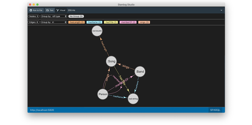
The simplest elements of the schema are Classes and Relationships. Classes are the distinct concepts that are represented. Relationships are how those classes are related. There are also Datatype Properties, the basic information or descriptors about an spefic instance of a class (e.g. age or serial number).

As you can see in the image, we have a basic schema. There are three classes: Person, Band, and Song. There are two relationships between them: memberOf and sings. A Person can be a memberOf a Band. Both a Person and a Band can sing a Song. There are also the Datatype Properties :hasLength, :hasName, and :hasTitle.

A relational aside

For those familiar with relational databases, we can already see a benefit of using the graph-based model. In a relational system, it is straightforward to model people, bands, songs, and that people are in bands. The schema would look something like this:

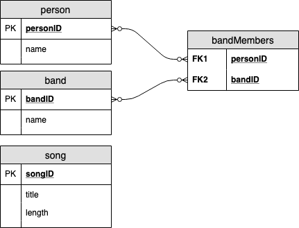
But how do we augment this to allow both a person and a band to sing songs?

• We could make separate bandSong and personSong tables and then have a view across them.
• We could create a concept of a performers table which has both a performerID value and a column for performerType (band or person).
• We could have a songPerformers table that has songID, performerID, and then typeID

All of these are reasonable and depend on what we want to do now and expect down the road, but we have to choose one. With our graph database, we don’t have to make this choice, and our schema much more closely matches our intuition and what we would draw on the whiteboard.

Query 1: Counting classes

Now, let’s run some top-level queries to explore the underlying data. Don’t worry about the queries themselves for now, just paste them in to the query workspace and hit Run. Make sure the database selected is GettingStarted_Music and the language of the query window, chosen in the bottom right, is SPARQL.

SELECT ?class (COUNT(?subject) as ?classCount)
WHERE {
    ?subject ?predicate ?object.
    ?subject rdf:type ?class .
}
GROUP BY ?class
ORDER BY DESC(?classCount)

This shows us all the classes and how many times each type of class appears. Note there will also be rows for rdf:Class and rdf:Property along with the Song, Band, and Person classes from above. This is a result of exactly how the data is stored, but you can ignore that for now.

Query 2: Counting relationships

SELECT ?predicate (COUNT(?predicate) as ?predicateCount)
WHERE {
    ?subject ?predicate ?object .
}
GROUP BY ?predicate
ORDER BY DESC(?predicateCount)

This shows us all the relationships and how many times each type of relationship appears. Like with our classes, there will be some things that are likely less familiar like rdf:type - gloss over them for now and look at things like :sings and :hasName.

Query 3: Sample data

SELECT *
WHERE {
    ?s ?p ?o .
}
LIMIT 100

This shows us 100 sample triples from the data, each that is of the form [Concept] → [Relationship] → [Concept]. So the first line we have shows that [David Bowie] → [rdf:type (aka is of type)] → [Person]. Your 100 rows may be different, and you may have to look down a few rows to see some actual people, bands, or songs.

This is common type of query to say “just give me some sample data”, which looks like this (and is often said as “Select S P O”). Make sure to include a LIMIT when you use it.

SPARQL 101

OK, enough taking our word for it, let’s start dissecting the queries a bit more as we run them. We’ll be writing queries in SPARQL, one of the most common languages for querying graphs. We’ll focus on the SELECT query, though there are a few other query types we’ll explore later on.

SELECT queries start by selecting triples in the graph to match. Once you have those triples back, you can aggregate them, filter them, all sorts of good things. But first, you have to say what data you want.

Query 4: Using variables to query

Let’s say we want all the songs that James Taylor sings. The query for that is

SELECT ?song
WHERE {
    :James_Taylor :sings ?song .
}

The part in the curly braces describes the data we want to return. :James_Taylor :sings ?song is called a triple pattern, which is essentially a triple where some of the elements may be variables. One or more triple patterns together form a basic graph pattern aka a BGP. In this case, the BGP is “data that looks like ‘James Taylor sings [something]’ “. Variables begin with a question mark, like ?song. We use the ?song variable within the braces and after SELECT to show that’s the specific data we want to see.

Query 5: Multiple variables in a triple pattern

In this dataset, we have only information about who sings songs - not who wrote them. If our dataset had information about writers and we wanted to to see all of James Taylor’s relationships with songs, this would be the query:

SELECT ?relationship ?song
WHERE {
    :James_Taylor ?relationship ?song .
}

If you run this, you’ll still get all the songs he sings, but you’ll also see an rdf:type result and a :hasName result. “But those aren’t songs - what’s going on?!” Let’s talk about variable names for a second (please, contain your excitement).

Just like in any programming or query languages, good variable names are helpful for readbility but do not actually change anything under the hood. So even though the above query has ?song as the variable name, there is nothing in the query that ensures it is actually a song (more on how to do that in query 7). So this query returns any triple with :James_Taylor as the subject. Best practice is to use a variable name that represents what you expect that variable to be - since the relationship is a variable here, the object could be anything, so instead of ?song, it would be clearer to call our variable ?object.

Query 6: Variable as the subject

Anything in the triple pattern can be a variable. We started with the object as the variable in query 4, then both the predicate and the object as variables in query 5. This query has the subject and the predicate as the variables.

By replacing :James_Taylor with ?performer and ?relationship with :sings, we’ll return combinations of any performer and their song. You must also add ?performer to the list of variables to SELECT - otherwise the query will just return the song names. The LIMIT 100 restricts the results to a manageable size.

SELECT ?performer ?song
WHERE {
?performer :sings ?song .
}
LIMIT 100

Query 7: More than one triple pattern

It gets interesting when we start to add more triple pattern. In query 5, we weren’t able to guarantee that the variable ?song returned a song. The query to do that looks like this:

SELECT *
WHERE {
    :James_Taylor ?relationship ?song .
    ?song a :Song.
}

This query says “Find me everything James Taylor is involved with” and then “Oh by the way, make sure that thing he’s involved with is a :Song.” So it will return only the Songs that he was involved with.

Because we SELECT *, we get back both the song and his relationship to it. If we wanted only the songs, we could write the first line as SELECT ?song.

This is the first query with more than one triple pattern. The period after the first triple pattern says that the next triple pattern is a new triple pattern with a full subject, object, and predicate. SPARQL syntax includes shorthand for situations where the subject or subject and object are repeated, but while you’re starting out, it’s helpful to write out each triple pattern fully and end each with a period. Technically you can omit the very last period, but the time savings of not typing a period is far outweighed by the cost of changing your query and then having the lack of period be an error. So please, use full triple patterns and periods every time!

Query 8: Aggregations and filters

In general, SPARQL supports a lot of the filter and aggregations you expect with any query language. So it looks more or less like what you’d expect to say “How many total songs did each person or band sing of at least 120 seconds”:

SELECT ?performer (COUNT(?song) as ?songCount)
WHERE {
    ?performer :sings ?song .
    ?song :hasLength ?length .
    FILTER (?length >= 120)
} GROUP BY ?performer
ORDER BY DESC(?songCount)

Inside the curly braces we’re saying “Find me every time any person or band sings a song, and make sure to also grab the length of those songs. But actually, I only want songs that are at least 120 seconds”. Then outside the curly braces we’re saying “count the number of songs grouped by the performer and sort descending by the number of matching songs.” And voila!

Another fun syntax note: SPARQL is case-sensitive. So if your second triple pattern is ?song :haslength ?length with a lowercase l, you will not get any results!

Exercise 1: Bands only

As an exercise, change Query 8 so that it only returns performers that are bands. You should get 32 results.

SELECT ?performer (COUNT(?song) as ?songCount)
WHERE {
    ?performer :sings ?song .
    ?song :hasLength ?length .
    ?performer a :Band .
    FILTER (?length >= 120)
} GROUP BY ?performer
ORDER BY DESC(?songCount)

Query 9: Queries with joins

Let’s find everyone who sings their own song and is also a member of a band (remember that this is an example dataset, so don’t be surprised when you see only Paul McCartney and Phil Collins!)

SELECT ?singer ?song
WHERE {
    ?singer :sings ?song .
    ?singer :memberOf ?band .
}

It is important that the ?singer variable in the first triple pattern is and the same as the ?singer in the second triple pattern. So what this is saying is “Find me a person who sings a song. Also, make sure that same person is in a band”. Note that you could reverse the order of the lines to get the same results:

SELECT * {
   ?singer :memberOf ?band .
   ?singer :sings ?song .
}

Query 10: Filter Not Exists

If we want to do the opposite of the above and find singers who are not in bands, we have to use a FILTER NOT EXISTS clause.

SELECT ?singer ?song {
    ?singer :sings ?song .
    FILTER NOT EXISTS {
    ?singer :memberOf ?band . }
}

This says “find me every singer and the songs they sing” and then “make sure I can’t find any examples of them being in a band.”

Exercise 2: Filter Not Exists

As a last exercise, try to write a query that finds all songs by performers (a band or a singer) who sing short songs - i.e. they haven’t written any songs longer than 240 seconds. Note that a FILTER NOT EXISTS clause is bound by curly braces (because it encloses a BGP) but a regular FILTER is bound by standard parentheses (because it is an operation on variable values).

You should get 18 results.

SELECT ?performer ?song {
    ?performer :sings ?song .
    FILTER NOT EXISTS {
        ?performer :sings ?anySong.
        ?anySong :hasLength ?length .
        FILTER (?length > 240)
    }
 }
 ORDER BY ?performer

One key part of this query is insuring the ?anySong variable is different than the first song variable - otherwise the query will be the same as finding songs that are not longer than 240 seconds.

What’s next?

That’s it for Getting Started: Part 1.

• To continue on with the Getting Started series, head on over to Getting Started: Part 2.
• For more SPARQL examples and practice, see our longer SPARQL Tutorial