Getting Started Part 4: Learn SPARQL in Studio
Put Knowledge Graph concepts in action using SPARQL
Page Contents
Introduction
This is part of the Stardog Getting Started series, which puts Knowledge Graph concepts in action. This tutorial introduces the SPARQL query language. We’ll start briefly in Explorer but work primarily in Studio.
Before you dive in, the introduction to the Getting Started series, Getting Started: Part 1 is a good pre-read.
This tutorial corresponds to Stardog’s SPARQL Tutorial knowledge kit.
Getting Started
To view the data for this Kit, click “Open in Explorer” under Try It Out. This opens a read-only view so you can inspect the schema and browse sample instance data—no install required. In Explorer, click Search with an empty Search bar to see the data model. You should see something like this:

When you’re ready to run your own SPARQL queries, click “Open in Studio” under Try It Out.
Understanding the Schema
In this guide we’ll use the term “schema”, but you may hear terms like “data model” and “ontology” that all mean approximately the same thing - what kind of information is represented in the data and how is it related.
The simplest elements of the schema are Classes and Relationships. Classes are the distinct concepts that are represented. Relationships are how those classes are related. There are also Datatype Properties, or Attributes, the basic information or descriptors about an specific instance of a class (e.g. age or serial number).
In this example, you’ll see our basic concepts, such as Band and Album, and their relations to other concepts, e.g. Bands are the artist for Albums and those Albums have via track a Track list. The attributes, such as an Album’s release year are not pictured in Explorer, you will see those in Designer, which is our tool for building Knowledge Graphs.
A relational aside …
For those familiar with relational databases, we can already see a benefit of using the graph-based model. In a relational system, it is straightforward to model people, bands, songs, and that people are in bands. The part of the schema would look something like this:
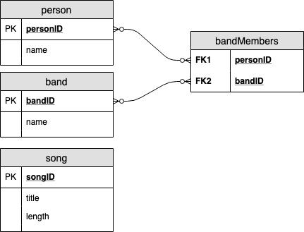
And some example data points would look like this:
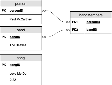
But how do we augment this to allow both a person and a band to sing songs?
- We could make separate bandSong and personSong tables and then have a view across them.
- We could create a concept of a performers table which has both a performerID value and a column for performerType (band or person).
- We could have a songPerformers table that has songID, performerID, and then typeID
All of these are reasonable and depend on what we want to do now and expect down the road, but we have to choose one. With our graph database, we don’t have to make this choice, and our schema much more closely matches our intuition and what we would draw on the whiteboard.
Using Studio
Now that we’ve explored this data a bit in Explorer to learn what it looks like, it’s time to learn SPARQL. For this, click “Open in Studio” under Try It Out to jump over to Studio.
Then, select the graph stardog-tutorial:music:music_data to ensure all of the queries you run are against the correct graph. It should look like this:
You can now copy any query from this tutorial, paste it into Studio, and click on “Run” to visualize your results.
Please note that you will need to ensure the SPARQL type (bottom right) is selected for your Editor Tab.
Introduction to SPARQL
Stardog Knowledge Graph supports the SPARQL query language, a W3C standard for querying RDF graphs. In Getting Started Part 3, we learned how to create a knowledge graph, and in this tutorial we will learn how to query them.
SELECT Queries
The main query form in SPARQL is a SELECT query which, by design, looks a bit like a SQL query. A SELECT query has two main components - a list of selected variables and a WHERE clause for specifying the graph patterns to match:
SELECT <variables>
WHERE {
   <graph-pattern>
}
The result of a SELECT query is a table where there will be one column for each selected variable and one row for each pattern match.
Triple Patterns
The basic building block for SPARQL queries is triple patterns. A triple pattern is just like an RDF graph triple, but you can use a variable in any one of the three positions. We use triple patterns to find the matching triples in a graph and variables act like wildcards that match any node.
For example,
# 01a-albums.sparql
prefix : <http://stardog.com/tutorial/>

SELECT ?album
WHERE {
   ?album rdf:type :Album .
}
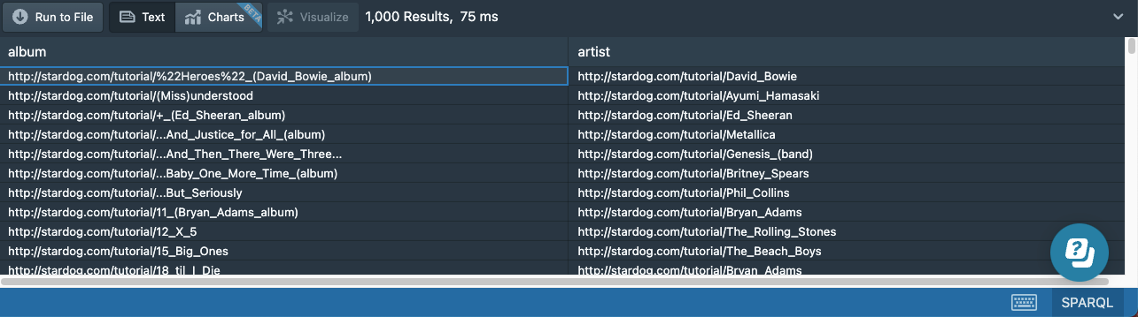
Here we see a simple SELECT query with a single triple pattern: ?album rdf:type :Album.
Stardog stores namespaces in database metadata, so we do not need to include the prefix declarations for every query.
This triple pattern will match all the triples in the graph that have rdf:type as the predicate and :Album as the object. The result set will look something like this:
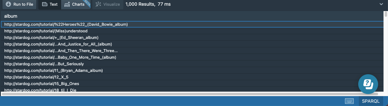
The column is only called album because that is what we called the variable. Naming variables like this, in an easy-to-understand way, is good practice, but be aware that your variables will be whatever you call them:
# 01b-bad-variable-name.sparql
prefix : <http://stardog.com/tutorial/>

SELECT ?bad_variable_name
WHERE {
   ?bad_variable_name rdf:type :Album .
}
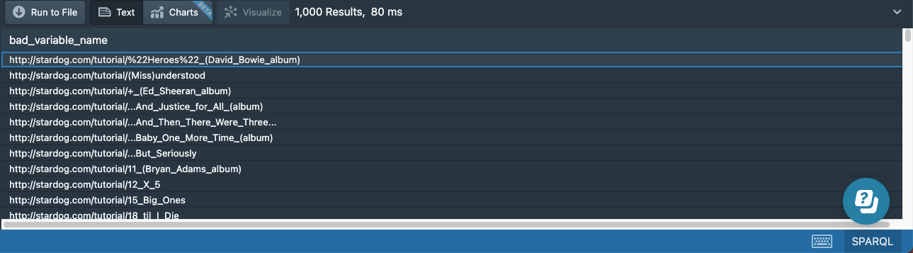
Your results might look different than the above table because there is no built-in ordering for query results in SPARQL. Note this dataset contains more than 1000 albums, but Studio limits result sets to 1000 results by default. You can see how to change this in Limiting Results.
There are several syntactic simplifications we can do to our original query (query 01a):
- the
WHEREkeyword is optional forSELECTqueries and can be omitted - if all the variables are being selected, then
*can be used instead of enumerating them explicitly - just like in RDF, the keyword
acan be used instead ofrdf:type - we can omit the trailing
.for the last triple pattern
If we apply all these simplifications, we get the following equivalent query, which we show on one line here to emphasize its concision:
# 01c-albums.sparql
prefix : <http://stardog.com/tutorial/>

SELECT * { ?album a :Album }
SPARQL keywords are case-insensitive, so one can use lowercase keywords like select instead of SELECT. We recommend consistency.
Basic Graph Patterns
When one or more triple patterns are used together, they form what is known as a Basic Graph Pattern (BGP). Let’s add one more triple pattern to our previous query to retrieve the artist for each album:
# 02-albums-artists.sparql
prefix : <http://stardog.com/tutorial/>

SELECT *
{
   ?album a :Album .
   ?album :artist ?artist .
}
The second triple pattern in this query will match the triples with :artist predicate, and we will get a result table with two columns:
Now let’s add a third triple pattern to require that the returned artists should be of the SoloArtist type:
# 03-albums-solo-artists.sparql
prefix : <http://stardog.com/tutorial/>

SELECT *
{
   ?album a :Album .
   ?album :artist ?artist .
   ?artist a :SoloArtist .
}
The third pattern matches 276 triples in our graph by itself, but because some solo artists have put out more than one album, 604 results are returned:
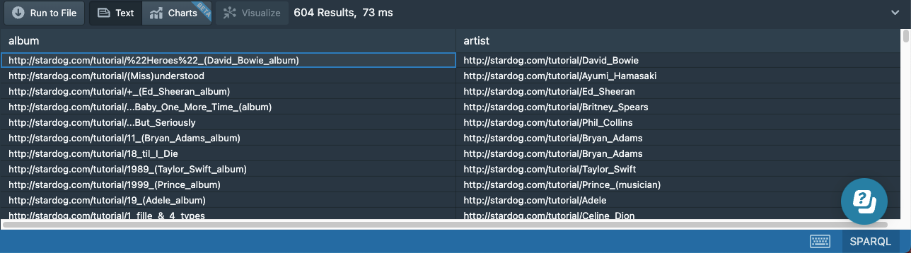
It’s good practice to have IRIs that are unique, persistent, and not too specific. In a production dataset, an IRI for an artist might be http://stardog.com/tutorial/74978455, and that IRI would have an rdfs:label of http://stardog.com/tutorial/David_Bowie. This dataset uses specific IRIs instead to make the tutorial more accessible to beginners.
Ordering Results
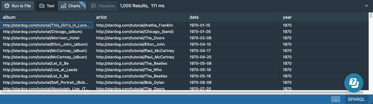
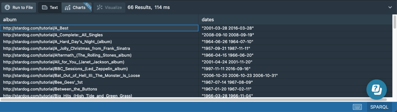
Now we’ll run the following query, which includes album dates:
# 04a-albums-dates.sparql
prefix : <http://stardog.com/tutorial/>

SELECT *
{
   ?album a :Album ;
          :artist ?artist ;
          :date ?date .
}
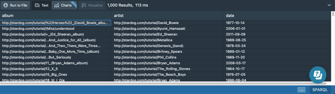
In this query, we used ; to separate triple patterns that share the same subject. In other words, the above query is equivalent to this query:
# 04b-albums-dates.sparql
prefix : <http://stardog.com/tutorial/>

SELECT *
{
   ?album a :Album .
   ?album :artist ?artist .
   ?album :date ?date .
}
You can see the results below:
If we want the results to be ordered based on a sorting condition, we can add an ORDER BY:
# 05-albums-dates-sorted.sparql
prefix : <http://stardog.com/tutorial/>

SELECT *
{
   ?album a :Album ;
          :artist ?artist ;
          :date ?date .
}
ORDER BY ?date
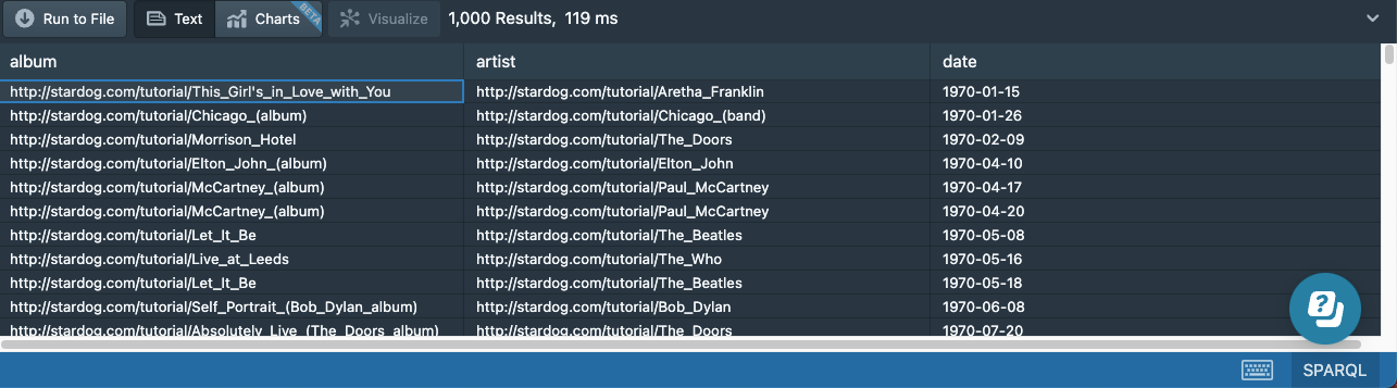
Now albums will be returned ordered by their release dates:
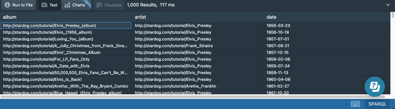
It is possible to have multiple sorting conditions by specifying multiple variables (or even function calls) in ORDER BY. We can also sort the results in descending order by encapsulating the sort condition with the DESC keyword, like this: DESC(?date).
Limiting Results
When a query returns too many results, we can limit the results with the LIMIT keyword:
# 06a-albums-dates-limited.sparql
prefix : <http://stardog.com/tutorial/>

SELECT *
{
   ?album a :Album ;
          :artist ?artist ;
          :date ?date
}
ORDER BY desc(?date)
LIMIT 2
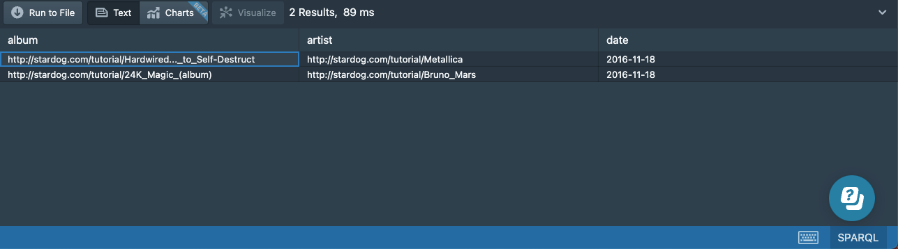
In this query, we changed the dates to be sorted in reverse chronological order and limited the query to return only two results:
You can override Studio’s default limit of 1000 by specifying a limit higher than 1000:
# 06b-albums-dates-bigger-limit.sparql
prefix : <http://stardog.com/tutorial/>

SELECT *
{
   ?album a :Album ;
          :artist ?artist ;
          :date ?date
}
ORDER BY desc(?date)
LIMIT 2000
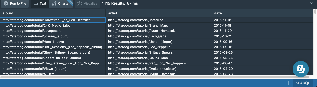
There are not 2000 triples that match this query, so the query will return the entire result set of 1,115 triples:
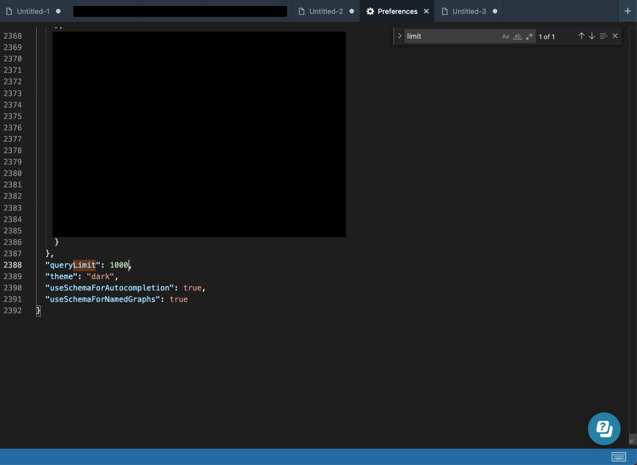
You can change Studio’s default query limit by opening Preferences (Cmd + , on Mac and Ctrl + , on Windows) and editing the value of queryLimit.
We can skip the first N results by adding an OFFSET N clause at the end of the query where N is a positive integer. A paging capability can be supported by using LIMIT and OFFSET.
Filtering Results
We can filter the results returned by a query using a FILTER expression. SPARQL supports many built-in functions for writing such expressions:
- comparison operators: (
=,!=,<,<=,>,>=) - logical operators (
&&,||,!) - mathematical operators (
+,-,/,*)
Plus many others. Stardog also provides an extensive number of additional functions.
If we want to find the albums released in 1970 or later, we can do this with the following filter expression:
# 07a-albums-dates-filtered.sparql
prefix : <http://stardog.com/tutorial/>

SELECT *
{
   ?album a :Album ;
          :artist ?artist ;
          :date ?date
   FILTER (?date >= "1970-01-01"^^xsd:date)
}
ORDER BY ?date
All otherwise matching results not satisfying the filter condition will be excluded from the results:
We can use any SPARQL function in the FILTER expressions. For example, the year function applied to a date value will return the year component as an integer value. So the following query will return the exact same results as the previous query, but the filter is written in a slightly different way:
# 07b-albums-dates-filtered.sparql
prefix : <http://stardog.com/tutorial/>

SELECT *
{
   ?album a :Album ;
          :artist ?artist ;
          :date ?date
      FILTER (year(?date) >= 1970)
}
ORDER BY ?date
Binding Values
We can assign the output of a function to a variable using the BIND keyword. This might be useful if we want to reuse the function result in different parts of the query or if we want to increase readability when we have a lot of nested function calls.
We can rewrite the previous query by binding the output of the year(?date) expression to a new variable ?year first and using the variable in the filter expresion:
# 07c-albums-dates-filtered.sparql
prefix : <http://stardog.com/tutorial/>

SELECT *
{
   ?album a :Album ;
          :artist ?artist ;
          :date ?date
   BIND (year(?date) AS ?year)
   FILTER (?year >= 1970)
}
ORDER BY ?date
Because we’re selecting all variables with *, the new variable we’ve bound will add another column to the output:
Removing Duplicates
Our music dataset is not complete by any means, and we have about a thousand albums. Suppose we want to find out the years in which these albums were released. One attempt would be to take the previous query, remove the filter, and only select the ?year variable.
# 08a-albums-years-duplicates.sparql
prefix : <http://stardog.com/tutorial/>

SELECT ?year
{
   ?album a :Album ;
          :artist ?artist ;
          :date ?date
   BIND (year(?date) AS ?year)
}
ORDER BY ?date
But we will quickly discover that this query will still return many results, and the year values will be repeated:
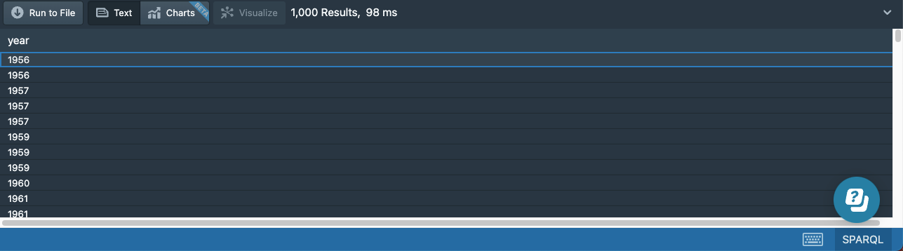
We can see that changing just the selected variables has no effect on the number of results returned by a query. We will still get one result for each matching pattern, so the number of rows in the result table won’t change; only the number of columns will change.
In order to get rid of duplicates, we need to use the DISTINCT keyword right after SELECT:
# 08b-albums-years-distinct.sparql
prefix : <http://stardog.com/tutorial/>

SELECT DISTINCT ?year
{
   ?album a :Album ;
          :artist ?artist ;
          :date ?date
   BIND (year(?date) AS ?year)
}
ORDER BY ?year
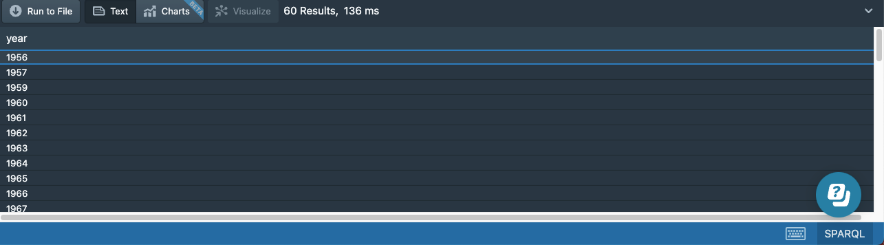
The results won’t have duplicates anymore:
Aggregation
Aggregation is applying a function to a list of values rather than to a single value. Unlike regular functions, aggregate functions can only be used in SELECT expressions. Built-in aggregates provided in SPARQL are COUNT, SUM, MIN, MAX, AVG, GROUP_CONCAT, and SAMPLE.
We can find the earliest and the latest release dates of albums in our dataset by using the MIN and MAX aggregates:
# 09-albums-dates.minmax.sparql
prefix : <http://stardog.com/tutorial/>

SELECT (min(?date) as ?minDate) (max(?date) as ?maxDate)
{
    ?album a :Album ;
           :date ?date
}
We will get a single result with two columns:
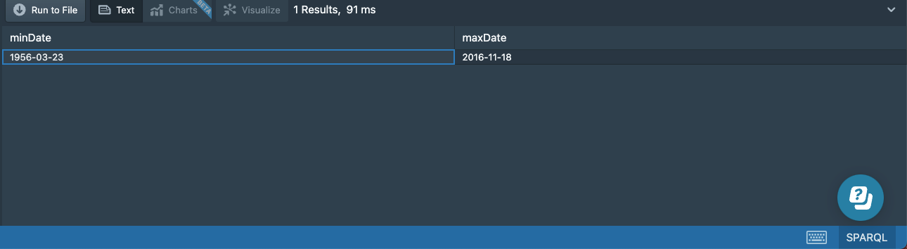
The WHERE clause in this query would return a table with two columns and many rows if we didn’t use the aggregate functions. The MIN (respectively, MAX) function looks at the values in the specified column of the results table and returns the single smallest (respectively, largest) value found.
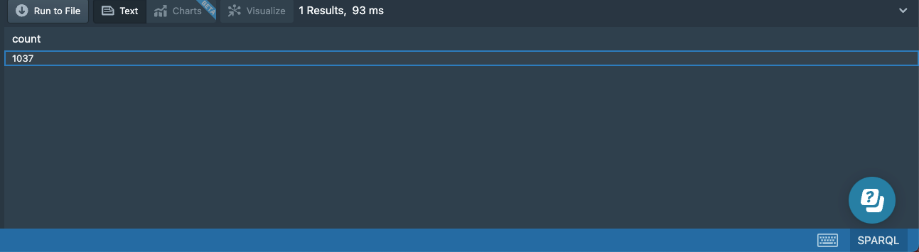
We can use the COUNT function to return the number of rows in the result table. The query to find the number of albums in our dataset is this:
# 10a-albums-count.sparql
prefix : <http://stardog.com/tutorial/>

SELECT (count(?album) as ?count)
{
    ?album a :Album
}
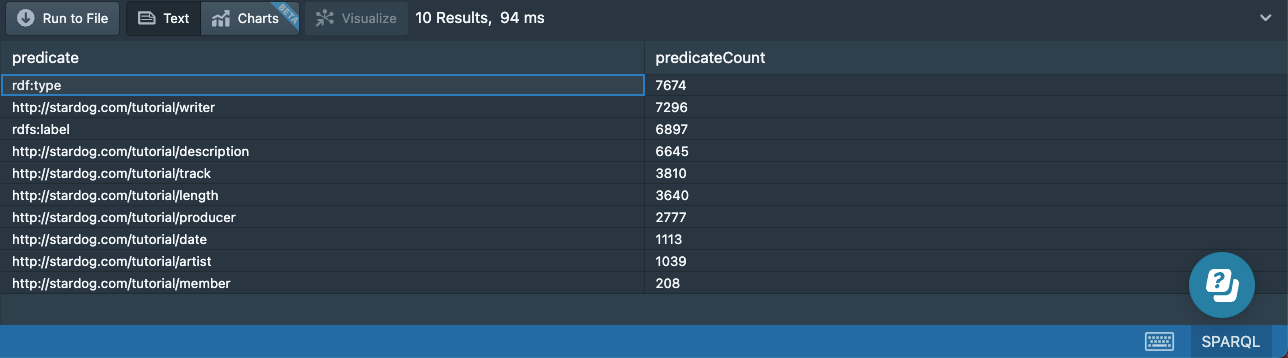
You can also count the relationships and how many times each type of relationship appears.
# 10b-predicate-count.sparql
prefix : <http://stardog.com/tutorial/>

SELECT ?predicate (COUNT(?predicate) as ?predicateCount)
{
    ?subject ?predicate ?object .
}
GROUP BY ?predicate
ORDER BY DESC(?predicateCount)
Another aggregation is sample data:
# 10c-sample-data.sparql
prefix : <http://stardog.com/tutorial/>

SELECT *
{
    ?s ?p ?o .
}
LIMIT 100
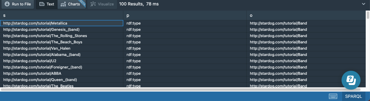
This shows us 100 sample triples from the data, each that is of the form [Concept] → [Relationship] → [Concept]. So the first line we have shows that [Metallica] → [rdf:type (aka is of type)] → [Band]. Your 100 rows may be different, and you may have to look down a few rows to see some actual people, bands, or songs.
This is common type of query to say “just give me some sample data”, which looks like this (and is often said as “Select S P O”). Make sure to include a LIMIT when you use it.
Grouping
The previous aggregation examples worked over a single result table and returned a single row as the final result. We can also group the results based on the values of one or more variables and apply the aggregation functions to each group separately.
Suppose we want to find the number of albums released each year. We can group the albums based on their release year and use the COUNT aggregate for each group:
# 11a-albums-dates-grouped.sparql
prefix : <http://stardog.com/tutorial/>

SELECT ?year (count(distinct ?album) AS ?count)
{
    ?album a :Album ;
            :date ?date ;
    BIND (year(?date) AS ?year)
}
GROUP BY ?year
ORDER BY desc(?count)
We will get one result for each distinct year value:
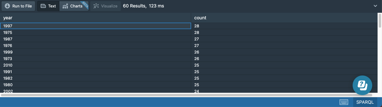
You might notice that we used the DISTINCT keyword inside the count aggregate. This is because some of the albums in our date have duplicate release dates. For example, the album “A Hard Day’s Night” has both 1964-06-26 and 1964-07-10 as release dates. This is due to the imperfection of our dataset, and using the DISTINCT keyword ensures we count the album only once for that year.
This is not a perfect solution since it means we’ll double count albums if their multiple release dates are in different years. It’s better to clean up the data. Fortunately, we can use the aggregates to find which albums have multiple release dates:
# 11b-albums-duplicate-dates.sparql
prefix : <http://stardog.com/tutorial/>

SELECT ?album (group_concat(?date) AS ?dates)
{
    ?album a :Album ;
            :date ?date
}
GROUP BY ?album
HAVING (count(?date) > 1)
The HAVING keyword we used at the end acts like an overall filter on the query results. Since the aggregates can only be used in SELECT expressions, we cannot use a regular FILTER (without introducing a subquery), so the HAVING keyword provides an easy way to define such filters.
Subqueries
If we want to find the average number of albums released in a year, we need to use an aggregation function over the results of the previous query. This can be achieved by subqueries where we simply put a SELECT query inside another one:
# 12-albums-dates-subselect.sparql
prefix : <http://stardog.com/tutorial/>

SELECT (avg(?count) AS ?avgCount)
{
      SELECT ?year (count(?album) AS ?count)
      {
            ?album a :Album ;
                  :date ?date ;
            BIND (year(?date) AS ?year)
      }
      GROUP BY ?year
}
The result of this query will be a single value:
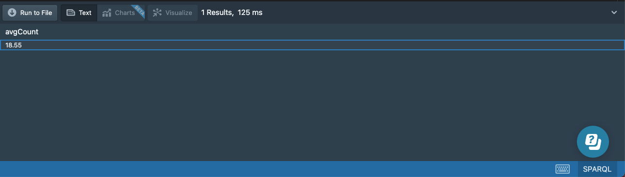
Of course, subqueries don’t have to use aggregation; it would be fine to use any kind of SELECT query as a subquery. If the outer WHERE clause contains additional patterns, then the subquery should be surrounded with {}.
Union
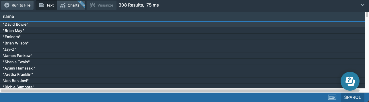
In our data, we have artists separated into two types: bands and solo artists. If we want to retrieve all artists along with their names, then we can use the UNION operator to combine the matches from two different patterns:
# 13a-artists-union.sparql
prefix : <http://stardog.com/tutorial/>

SELECT ?name
{
    { ?artist a :SoloArtist }
    UNION
    { ?artist a :Band }
    ?artist rdfs:label ?name
}
The results will contain artists matching either pattern:
If the same artists matched both patterns, we would get a duplicate result and need DISTINCT to get unique results.
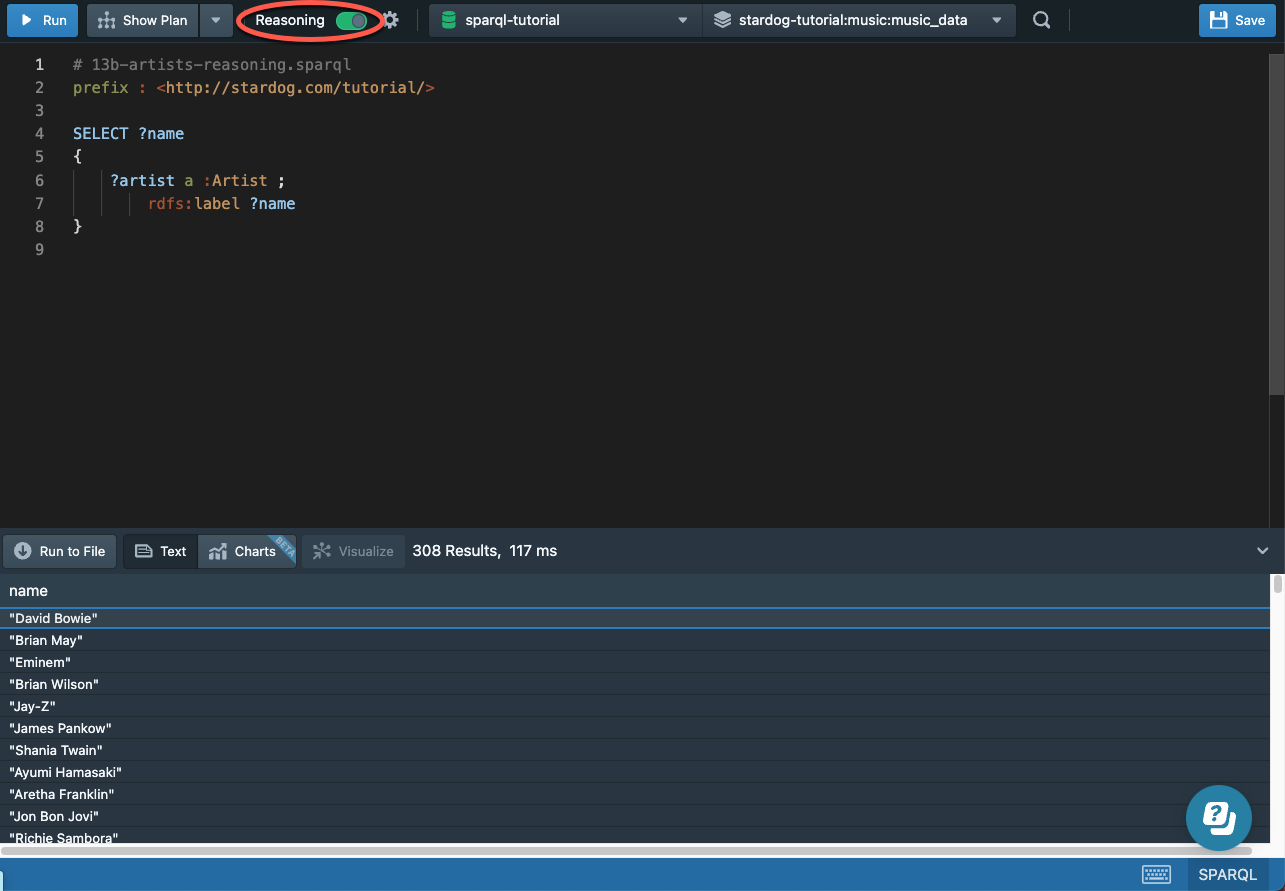
If we enable reasoning in our queries (by using the reasoning toggle button in Stardog Studio), we can write a much simpler query because :Band and :SoloArtist are subclasses of :Artist:
# 13b-artists-reasoning.sparql
prefix : <http://stardog.com/tutorial/>

SELECT ?name
{
    ?artist a :Artist ;
        rdfs:label ?name
}
And we can see our results are exactly the same:
To learn more about reasoning, see our Inference Engine tutorial.
Optional Matches
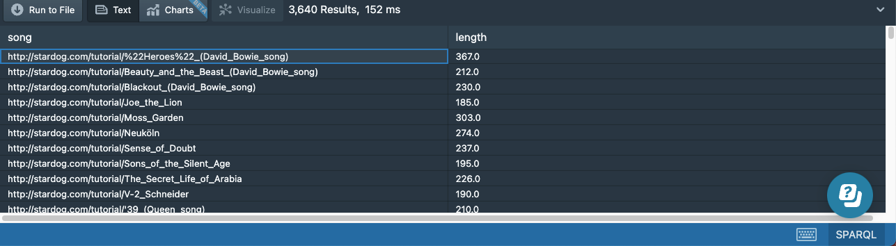
The following query returns the songs and their lengths:
# 14a-songs-length.sparql
prefix : <http://stardog.com/tutorial/>

SELECT *
{
    ?song a :Song .
    ?song :length ?length .
}
LIMIT 5000 # included to override default limit
When we look at the results, we see this query returns 3,640 results:
Whereas the query without the second pattern returns 3,749 songs:
# 14b-songs.sparql
prefix : <http://stardog.com/tutorial/>

SELECT *
{
    ?song a :Song .
}
LIMIT 5000 # included to override default limit
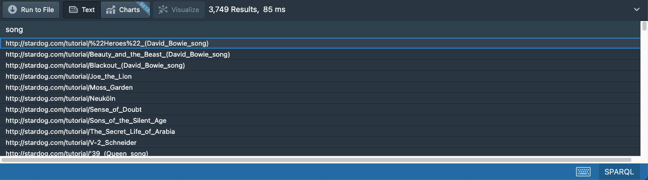
This means there are 109 songs in our dataset that do not have any length information.
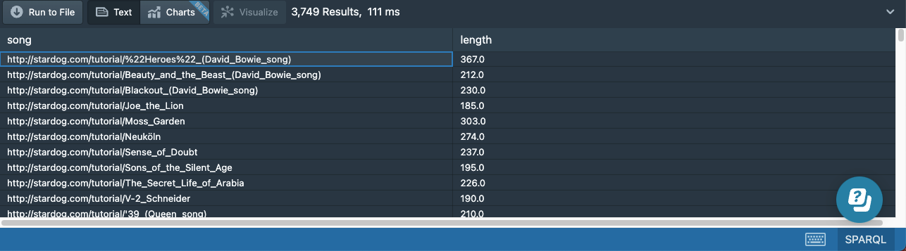
We can use OPTIONAL blocks to match patterns that may exist for some nodes but not for others:
# 14c-songs-optional-length.sparql
prefix : <http://stardog.com/tutorial/>

SELECT ?song ?length
{
    ?song a :Song .
    OPTIONAL {
        ?song :length ?length .
    }
}
LIMIT 5000 # included to override default limit
This query will return 3,749 results, where 109 rows will not have a value for the length:
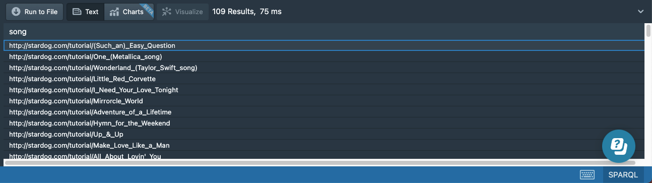
If we only want to see those rows where length is missing, we can add a filter to our query:
# 14d-songs-unbound-length.sparql
prefix : <http://stardog.com/tutorial/>

SELECT ?song ?length
{
    ?song a :Song .
    OPTIONAL {
        ?song :length ?length .
    }
    FILTER(!bound(?length))
}
And we get the 109 results we were expecting:

Negation
The last example shows a somewhat indirect way to find patterns that do not exist in the dataset by using a combination of OPTIONAL and FILTER expressions. But SPARQL provides a special kind of filter for this purpose: NOT EXISTS. The following query will return the same 109 results as the previous query:
# 14e-songs-no-length.sparql
prefix : <http://stardog.com/tutorial/>

SELECT ?song
{
    ?song a :Song .
    FILTER NOT EXISTS {
        ?song :length ?length .
    }
}
Any SPARQL construct can be used inside a NOT EXISTS block.
Property Paths
The triple patterns match triples in the dataset, so they can only be used to find nodes that are directly connected. We can use property paths to match nodes that are connected via arbitrary-length paths. More generally, a property path is a regular expression describing the possible route between two nodes in a graph. Property paths can also be used to express some graph patterns more concisely.
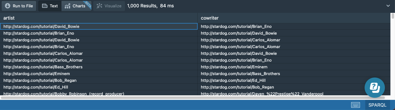
To explore what we can do with property paths we will start with this query that uses two ordinary triple patterns to find pairs of people who wrote songs together:
# 15a-cowriters.sparql
prefix : <http://stardog.com/tutorial/>

select distinct ?artist ?cowriter
{
    ?song :writer ?artist .
    ?song :writer ?cowriter
    FILTER (?artist != ?cowriter)
}

We need DISTINCT in this query because the same pair might have cowritten multiple songs together. We need the FILTER because otherwise the query would match the songs with a single writer and bind the two variables ?artist and ?cowriter to the same person. Using a different variable does not ensure that the triple patterns match different triples in the data. This query returns each pair twice; we leave it as an exercise to the reader to come up with a different filter expression to return every pair only once.
Inverse Path
Adding the symbol ^ in front of a predicate (or a property path expression) makes it an inverse path expression. An inverse path expression simply flips the direction of the match: the subject of the triple pattern will match the object of the triple in the data, and the object of the triple pattern will match the subject. So an equivalent way to write the previous query is as follows:
# 15b-cowriters-inverse-path.sparql
prefix : <http://stardog.com/tutorial/>

select distinct ?artist ?cowriter
{
    ?artist ^:writer ?song .
    ?song :writer ?cowriter
    FILTER (?artist != ?cowriter)
}

By itself, an inverse property path expression is not very useful, but in combination with other property path expressions, it can be (as we will see next).
Sequence Path
When the object of one triple pattern is the same as the subject of another triple pattern, and we are not interested in the binding of the variable, we can combine the two patterns using a sequence path. A sequence path means the subject is connected to the object via the path of property expressions specified in the sequence. The next query returns the same results as the previous query:
# 15c-cowriters-property-path.sparql
prefix : <http://stardog.com/tutorial/>

select distinct ?artist ?cowriter
{
    ?artist ^:writer/:writer ?cowriter
    FILTER (?artist != ?cowriter)
}
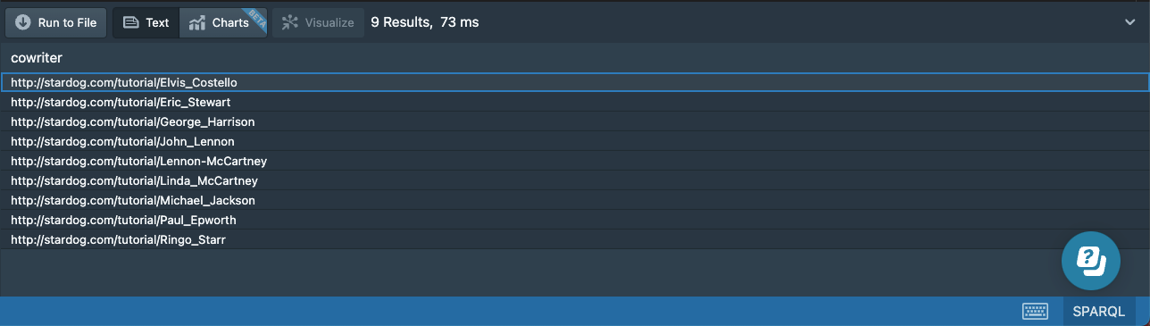
There can be more than two expressions in a path if necessary. We can also use constants for the subject or the object or both. The next query returns cowriters of Paul McCartney:
# 15d-cowriters-mccartney.sparql
prefix : <http://stardog.com/tutorial/>

select distinct ?cowriter
{
    :Paul_McCartney ^:writer/:writer ?cowriter
    FILTER (?cowriter != :Paul_McCartney)
}
order by ?cowriter
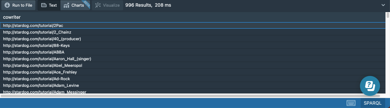
Recursive Paths
Suppose we want to find not only the cowriters of Paul McCartney, but also the cowriters of his cowriters, and continue finding cowriters recursively. We can use the recursive path operator + to follow a property path one or more times.
# 15e-cowriters-recursive.sparql
prefix : <http://stardog.com/tutorial/>

select distinct ?cowriter
{
    :Paul_McCartney (^:writer/:writer)+ ?cowriter
    FILTER (?cowriter != :Paul_McCartney)
}
order by ?cowriter
The other recursive operator, *, is used to follow a path zero or more times. Following a path zero times means we don’t traverse any edges and simply return the same node as the starting node. This makes most sense when used in a sequence path as in rdf:type/rdfs:subClassOf*. This property path returns the type(s) of a node and all its superclasses.
Optional Paths
In our dataset, we have both the solo albums released by Paul McCartney and the albums released by The Beatles. The next query would return both kinds of album:
# 15f-songs-optional-path.sparql
prefix : <http://stardog.com/tutorial/>

select ?album
{
  ?album :artist/:member? :Paul_McCartney
}

The ? suffix means we should follow a path zero or one times. The property path expression :artist/:member? would start with an album and first find all the nodes connected via the :artist predicate and return those nodes (since we would end up on those nodes when we follow the :member edge zero times). Then if any of those nodes have a :member edge, it will follow those edges and return the new nodes we reach as well.
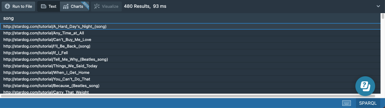
Alternative Paths
Suppose we want to find all the songs related to Paul McCartney: songs released in either his solo albums or The Beatles’ albums, along with the songs he wrote that were recorded by other artists. We need to find three alternate paths from songs to Paul McCartney. The previous property path expression already (partially) encodes two of these paths, and the third alternate path can be introduced using the | path operator:
# 15g-songs-alternative-path.sparql
prefix : <http://stardog.com/tutorial/>

select ?song
{
  ?song (^:track/:artist/:member?)|:writer :Paul_McCartney
}
Shortest Path Queries
As we have just seen, SPARQL property paths can be used to find pairs of nodes connected via a complex path of edges. But these property paths only return the start and end nodes of a path and not the intermediate nodes within the path.
In the Recursive Paths example, we have seen how we can recursively find all the nodes connected to Paul McCartney via cowriter relationships. When we run that query we can see in the results that Kanye West is connected to Paul McCartney, but there isn’t a song they cowrote together, and we can’t tell by looking at the results how they are connected. We can use path queries to get the answers.
Stardog path queries are an extension to SPARQL, and we can use them to find not only (shortest or all) paths between two nodes defined, but also to find all the intermediate nodes on that path. The connection between nodes can be a single property or a more complex SPARQL pattern.
The path query equivalent to the property path expression in 15e-cowriters-recursive.sparql is as follows:
# 16a-cowriters-paths.sparql
prefix : <http://stardog.com/tutorial/>

paths     start ?artist = :Paul_McCartney
    end ?cowriter
via {
    ?artist ^:writer/:writer ?cowriter
}
order by ?cowriter
The result of the query will be a list of paths:
The VIA clause in a path query is similar to a WHERE clause in a SELECT query, but instead of returning the matches for this pattern, a path query traverses this pattern in the graph recursively, starting with the start node until reaching the end node.
The start and end nodes in a path query can be completely unrestricted to find the shortest paths between any node in the graph, but such queries are typically intractable due to the very high number of such paths.
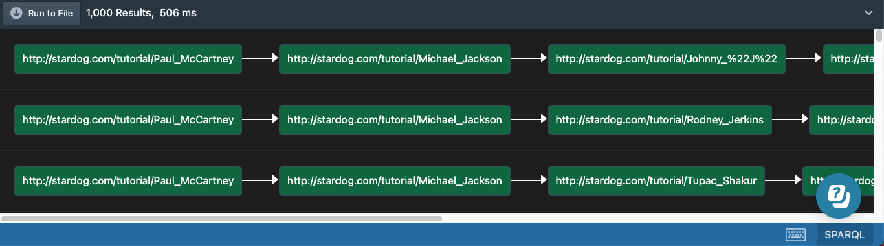
Now, if we want to see the paths between Paul McCartney and Kanye West, we can run the following query:
# 16b-cowriters-paths.sparql
prefix : <http://stardog.com/tutorial/>

paths     start ?artist = :Paul_McCartney
    end ?cowriter = :Kanye_West

via {
    ?song :writer ?artist .
    ?song :writer ?cowriter
}

order by ?cowriter
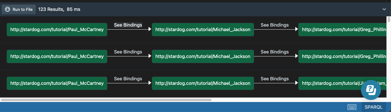
Note that in this version of the query, we are using an explicit variable for the song, so we can also see at each step of the path what song the cowriters collaborated on. You can see the song by clicking on “See Bindings”. The first path in the above screenshot, represented as text, looks as follows:
(:Paul_McCartney)-[song=:Say_Say_Say]->(:Michael_Jackson)-[song=:P.Y.T._(Pretty_Young_Thing)]->(:Greg_Phillinganes)-[song=:Love_Will_Conquer_All]->(:Cynthia_Weil)-[song=:Through_the_Wire]->(:Kanye_West)
Path queries are a powerful addition to SPARQL, and you can find more details about how to use them in the Stardog documentation.
SPARQL Query Forms
There are SPARQL query forms other than the SELECT queries. The WHERE clause in these queries can use any of the constructs we described above, but the query result will not be a table.
ASK Queries
Ask queries return a boolean result indicating if the pattern specified in the WHERE clause matched any result or not. The next query asks if there is any band credited as the writer of a song:
# 17-bands-writers-ask.sparql
prefix : <http://stardog.com/tutorial/>

ASK
{
    ?band a :Band .
    ?song :writer ?band .
}
The result is simply true without any detail about which song or band matches this pattern:

Since the ASK queries don’t return any bindings, they can be more efficient than executing a SELECT query.
DESCRIBE Queries
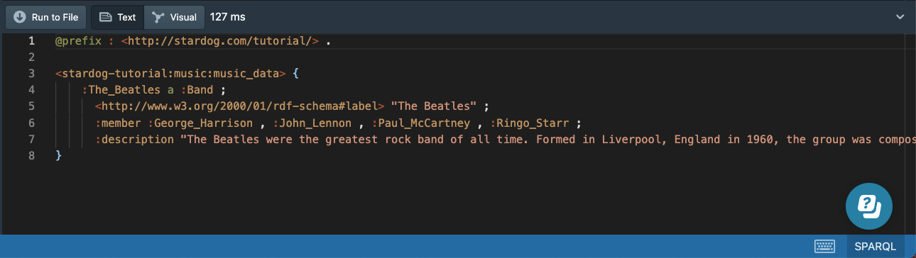
The DESCRIBE query returns an RDF graph. What triples are returned for a node is not prescribed in the SPARQL specification and is in fact system-dependent. The default DESCRIBE implementation in Stardog returns all the outgoing edges of the node:
# 18a-beatles-describe.sparql

PREFIX : <http://stardog.com/tutorial/>

DESCRIBE :The_Beatles
The resulting triples has :The_Beatles as the subject:
The DESCRIBE query is most useful when we don’t know anything about the RDF graph we are querying and want to quickly see the terms used in the triples. The query SELECT * { :The_Beatles ?p ?o } would serve the same purpose as the above query.
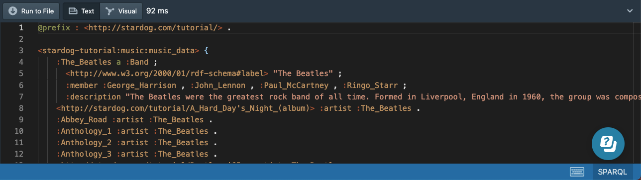
Stardog provides a special query hint to change the DESCRIBE strategy being used. The following query returns the incoming edges too:
# 18b-beatles-describe-bidirectional.sparql

PREFIX : <http://stardog.com/tutorial/>
#pragma describe.strategy bidirectional
DESCRIBE :The_Beatles
It is possible to specify a WHERE clause in a DESCRIBE query to describe the values bound to one or more variables. The following query will describe every band with a name starting with the word “The”:
# 18c-bands-describe.sparql

PREFIX : <http://stardog.com/tutorial/>

DESCRIBE ?band
{
    ?band a :Band ;
         rdfs:label ?name
    FILTER(contains(?name, "The"))
}
CONSTRUCT Queries
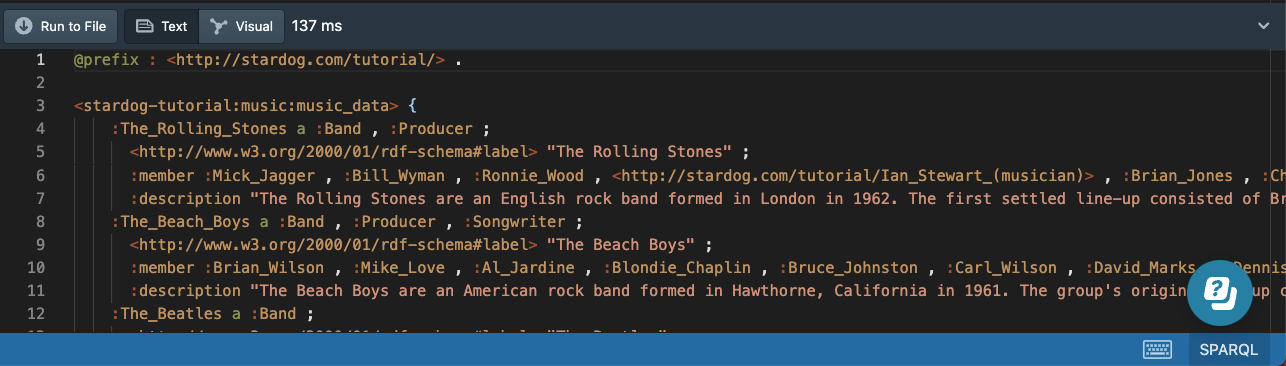
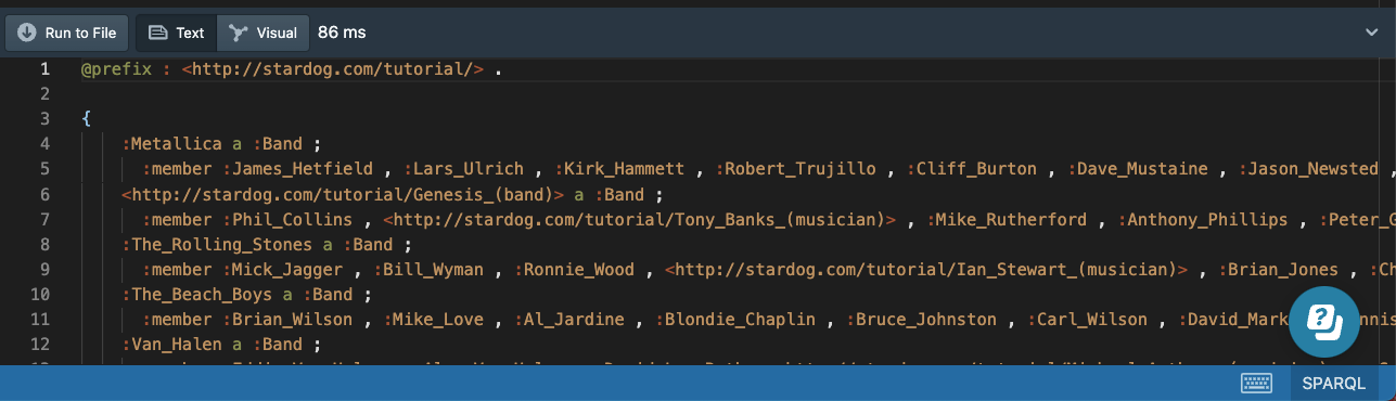
A CONSTRUCT query matches patterns in a WHERE clause and then returns an RDF graph as a result. If the WHERE clause only contains triple patterns, we can use the short-hand syntax; for example, to retrieve the bands and their members:
# 19a-bands-construct.sparql

PREFIX : <http://stardog.com/tutorial/>

CONSTRUCT
{
    ?band a :Band ;
          :member ?member
}
WHERE {
    ?band a :Band ;
        :member ?member
}
The result will look something like this:
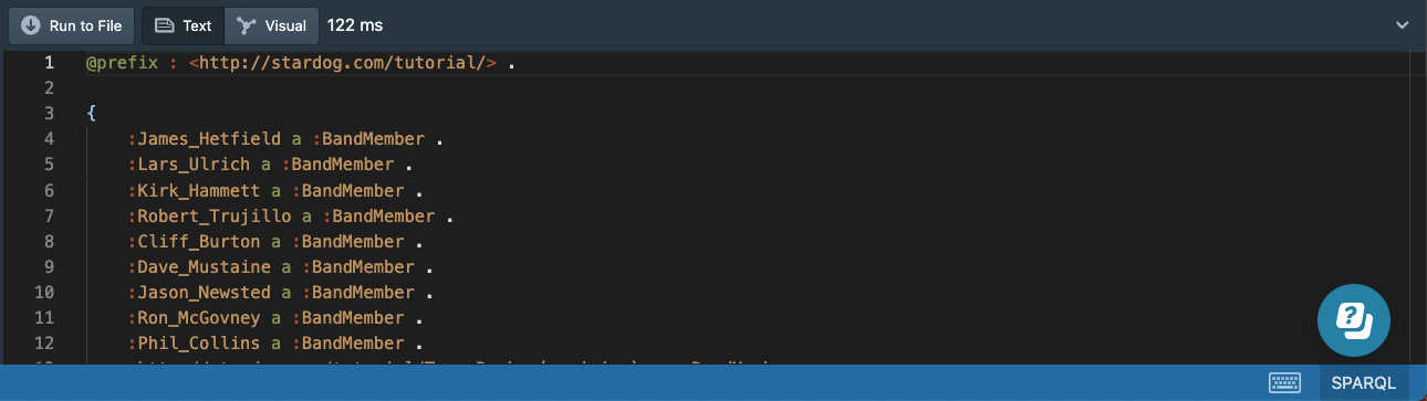
We can specify a CONSTRUCT template that will return a different set of triples than the triples we matched in the WHERE clause:
# 19b-bands-members-construct.sparql

PREFIX : <http://stardog.com/tutorial/>

CONSTRUCT {
    ?member a :BandMember
}
WHERE {
    ?band a :Band ;
          :member ?member
}
The triples returned for this query do not exist in our graph:
CONSTRUCT queries are read-only just like the other query forms we have seen so far and do not modify the input RDF graph. If we want to modify the RDF graph, we need to use SPARQL update queries that we discuss next.
Update Queries
Note: The example SPARQL queries and model creation steps shown below are read-only. Queries that insert, update, or modify data cannot be executed in this tutorial environment.
If we want to insert triples into the database based on the results of a query, we can use an INSERT query. The following query is similar to the above CONSTRUCT query but simply inserts the resulting triples into the database:
# 20-bands-members-insert.sparql
prefix : <http://stardog.com/tutorial/>

INSERT {
    ?member a :BandMember
}
WHERE {
    ?band a :Band ;
          :member ?member
}
We can change the INSERT to a DELETE to delete triples from the database.
In our graph, we used an integer range for the :length property to specify the length of a song in seconds. This is simple and good enough in most cases, but using the XML Scheme datatype xsd:dayTimeDuration is better, as it avoids the ambiguity of the time unit associated with the length. So if we want to replace all :length values in our data to use duration values, we can execute the following update query that will delete the existing triples with integer values and insert new triples with duration values:
# 21a-songs-length-delete.sparql
prefix : <http://stardog.com/tutorial/>

DELETE {
    ?song :length ?seconds
}
INSERT {
    ?song :length ?duration
}
WHERE {
    ?song a :Song ;
         :length ?seconds
    BIND(?seconds * "PT1S"^^xsd:dayTimeDuration AS ?duration)
}
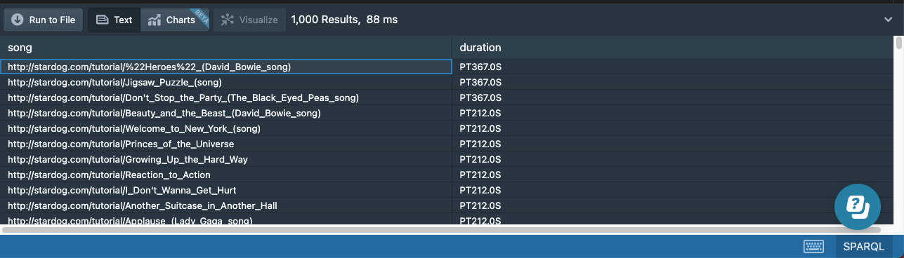
Because the output of a CONSTRUCT query is not very informative, we can use a SELECT query to confirm our data has been updated to our liking:
# 21b-songs-length-delete.sparql
prefix : <http://stardog.com/tutorial/>

SELECT * {
    ?song :length ?duration
}
What’s next?
That’s it for Getting Started: Part 4. To continue on with the Getting Started series, head on over to Getting Started: Part 5.