Reading Stardog Query Plans
Learn how to read Stardog query plans to write better queries.
Page Contents
Reading query plans is key to optimizing Stardog query performance. In this tutorial we teach you how to read and reformulate them. Learning how to read Stardog query plans is a great way to become more adept at writing more performant queries.
The “Syntax” of Query Plans
I am going to use the following running example to explain most things about query plans in Stardog. The query below is Q5b from the well-known SP2B SPARQL benchmark:
# Query 5b

SELECT DISTINCT ?person ?name
WHERE {
   ?article rdf:type bench:Article .
   ?article dc:creator ?person .
   ?inproc rdf:type bench:Inproceedings .
   ?inproc dc:creator ?person .
   ?person foaf:name ?name
}
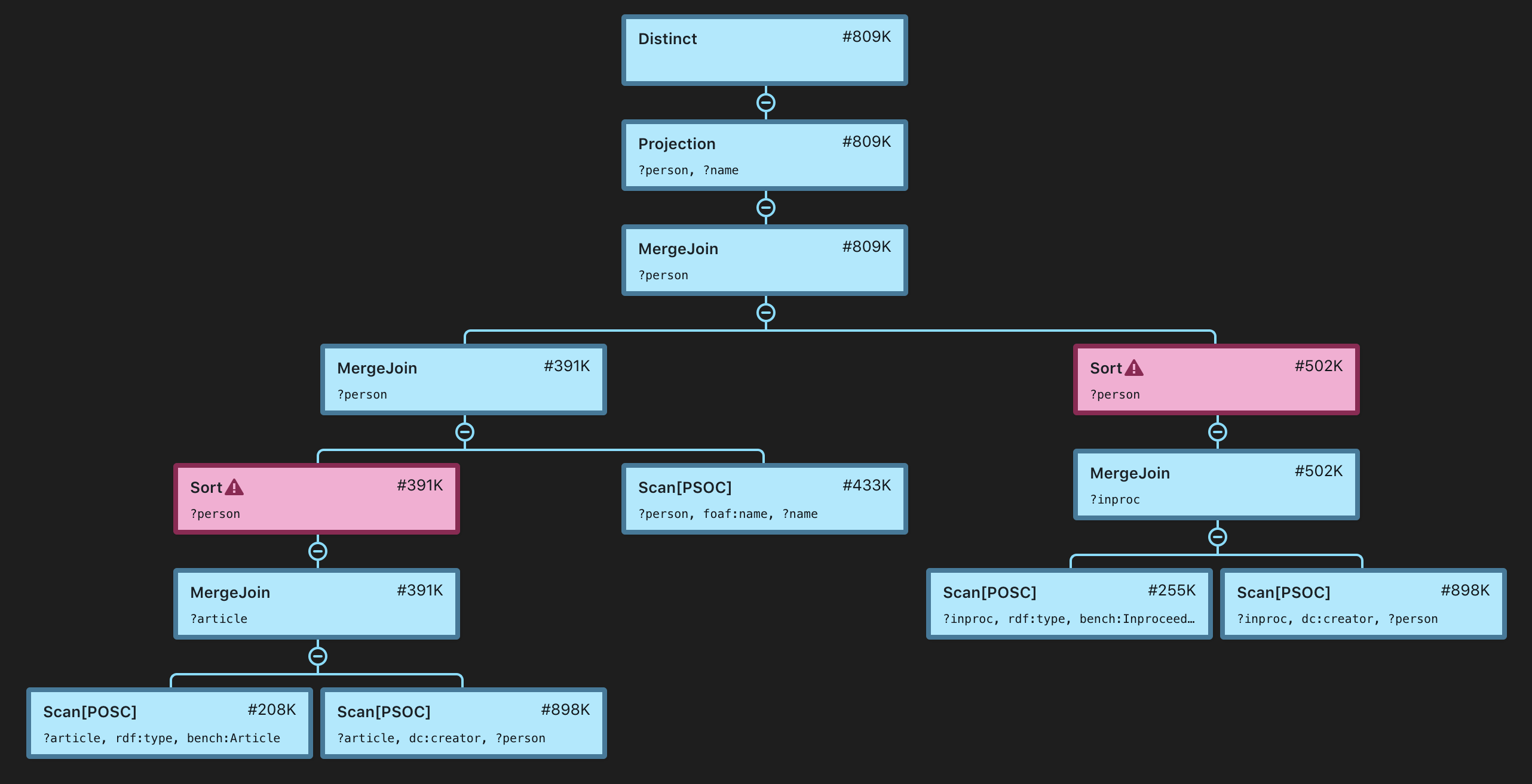
This query returns the names of all people who have authored both a journal article and a paper in a conference proceedings. The query plan used by Stardog 7.0.0 to evaluate this query is:
Distinct [#809K]
`─ Projection(?person, ?name) [#809K]
   `─ MergeJoin(?person) [#809K]
      +─ MergeJoin(?person) [#391K]
      │  +─ Sort(?person) [#391K]
      │  │  `─ MergeJoin(?article) [#391K]
      │  │     +─ Scan[POSC](?article, rdf:type, bench:Article) [#208K]
      │  │     `─ Scan[PSOC](?article, dc:creator, ?person) [#898K]
      │  `─ Scan[PSOC](?person, foaf:name, ?name) [#433K]
      `─ Sort(?person) [#502K]
         `─ MergeJoin(?inproc) [#502K]
            +─ Scan[POSC](?inproc, rdf:type, bench:Inproceedings>) [#255K]
            `─ Scan[PSOC](?inproc, dc:creator, ?person) [#898K]

As you can see, the plan looks like a hierarchical, tree-like structure. The nodes, called operators, represent units of data processing during evaluation. They correspond to evaluations of graphs patterns or solution modifiers as defined in the SPARQL 1.1 specification. All operators can be regarded as functions which may take some data as input and produce some data as output. All input and output data is represented as streams of solutions, that is, sets of bindings of the form x -> value where x is a variable used in the query and value is some RDF term (IRI, blank node, or literal). Examples of operators include scans, joins, filters, unions, etc.
Numbers in square brackets after each node refer to the estimated cardinality of the node, i.e. how many solutions Stardog expects this operator to produce when the query is evaluated. Statistics-based cardinality estimation in Stardog merits a separate blog post, but here are the key points for the purpose of reading query plans:
- all estimations are approximate and their accuracy can vary greatly (generally: more precise for bottom nodes, less precise for upper nodes)
- estimations are only used for selecting the best plan but have no bearing on the actual results of the query
- in most cases a sub-optimal plan can be explained by inaccurate estimations
Stardog Evaluation Model
Stardog generally evaluates query plans according to the bottom-up semantics of SPARQL. Leaf nodes are evaluated first and without input, and their results are then sent to their parent nodes up the plan. Typical examples of leaf nodes include scans, i.e. evaluations of triple patterns, evaluations of full-text search predicates, and VALUES operators.
They contain all information required to produce output, for example, a triple pattern can be directly evaluated against Stardog indexes. Parent nodes, such as joins, unions, or filters, take solutions as inputs and send their results further towards the root of the tree. The root node in the plan, which is typically one of the solution modifiers, produces the final results of the query which are then encoded and sent to the client.
Pipelining and Pipeline Breakers
Stardog follows the pipelined query execution model, also known as the Volcano Model, in which evaluation is as lazy as possible. Each operator does just enough work to produce the next solution. This is important for performance, especially for queries with a LIMIT clause (of which ASK queries are a special case) and also enables Stardog’s query engine to send the first result(s) as soon as they are available (as opposed to waiting till all results have been computed).
Not all operators can produce output solutions as soon as they get first input solutions from their children nodes. Some need to accumulate intermediate results before sending output. Such operators are called pipeline breakers, and they are often the culprits for performance problems, typically resulting from memory pressure. It is important to be able to spot them in the plan since they can suggest either a way to re-formulate the query to help the planner or a way to make the query more precise by specifying extra constraints where they matter.

Here are some important pipeline breakers in the example plan:
HashJoin: hash join algorithms build a hash table for solutions produced by the right operand. Typically all such solutions need to be hashed, either in memory or spilled to disk, before the first output solution is produced by theHashJoinoperator.Sort: the sort operator builds an intermediate sorted collection of solutions produced by its child node. The main use case for sorting solutions is to prepare data for an operator which can benefit from sorted inputs, such asMergeJoin,Distinct, orGroupBy. Of course all solutions have to be fetched from the child node before the smallest (w.r.t. the sort key) solution can be emitted.GroupBy: group-by operators are used for aggregation, e.g. counting or summing results. When evaluating a query like select ?x (count(?y) as ?count) where { ... } group by ?xStardog has to scroll through all solutions to compute the count for every?xkey before returning the first result.
Other operators can produce output as soon as they get input, most notably the following:
MergeJoin: merge join algorithms do a single zig-zag pass over sorted streams of solutions produced by children nodes and output a solution as soon as the join condition is satisfied.DirectHashJoin: contrary to the classical hash join algorithm, this operator does not build a hash table. It utilizes Stardog indexes for look-ups which doesn’t require extra data structures. This is only possible when the right operand is sorted by the join key, but the left isn’t, otherwise Stardog would use a merge join.Filter: a solution modifier which evaluates the filter condition on each input solution.Union: combines streams of children solutions without any extra work, e.g. joining, so there’s no need for intermediate results.
Now, returning to the above query, one can see Sort pipeline breakers in the plan:
Sort(?person) [#391K]
`─ MergeJoin(?article) [#391K]
   +─ Scan[POSC](?article, rdf:type, bench:Article) [#208K]
   `─ Scan[PSOC](?article, dc:creator, ?person) [#898K]
This means that all solutions representing the join of ?article rdf:type bench:Article and ?article dc:creator ?person will be put in a sequence ordered by the values of ?person. Stardog expects to sort 391K solutions before they can be further merge-joined with the results of the ?person foaf:name ?name pattern. Alternatively the engine could build a hash table instead of sorting solutions; such decisions are made by the optimizer based on a number of factors.
Skipping Intermediate Results
One tricky part of understanding Stardog query plans is that evaluation of each operator in the plan is usually context-sensitive, i.e. it depends on what other nodes are in the same plan, possibly in a different sub-tree. In particular, the cardinality estimations, even if assumed accurate, only specify how many solutions the operator is expected to produce when evaluated as the root node of a plan.
However, as it is joined with other parts of the plan, the results can be quite different. This is because Stardog employs optimizations to reduce the number of solutions produced by a node by pruning those which are incompatible with other solutions with which they will later be joined.

Consider the following basic graph pattern and the corresponding plan:
?erdoes rdf:type foaf:Person .
?erdoes foaf:name "Paul Erdoes"^^xsd:string .
?document dc:creator ?erdoes .
MergeJoin(?erdoes) [#294]
+─ MergeJoin(?erdoes) [#1]
│  +─ Scan[POSC](?erdoes, rdf:type, foaf:Person) [#433K]
│  `─ Scan[POSC](?erdoes, foaf:name, "Paul Erdoes") [#1]
`─ Scan[POSC](?document, dc:creator, ?erdoes) [#898K]
The pattern matches all documents created by a person named Paul Erdoes. Here the second pattern is very selective (only one entity is expected to have the name “Paul Erdoes”). This information is propagated to the other two scans in the plan via merge joins, which allows them to skip scanning large parts of data indexes.
In other words, the node Scan[POSC](?erdoes, rdf:type, foaf:Person) [#433K] will not produce all 433K solutions corresponding to all people in the database and, similarly, Scan[POSC](?document, dc:creator, ?erdoes) [#898K] will not go through all 898K document creators.
This is only one example of avoiding intermediate results. In combination with other optimizations, such as algebraic rewriting, Stardog can dramatically reduce the number of intermediate results.
It should be noted that this optimization interacts tightly with pipelined execution and is affected by pipeline breakers. The lazy evaluation model means that there’s usually only a limited amount of information available for optimization (since data isn’t accumulated in memory, whenever possible).

Pipeline breakers—e.g. sort nodes and hash joins—usually process unsorted data; that makes it difficult to take advantage of pruning. This means that usually hash joins hash the number of solutions which corresponds to cardinality of the right operand (modulo statistical inaccuracies) and, similarly, sort operators are expected to sort as many solutions as indicated for the child node. This simplifies plan analysis, i.e. the expected memory footprint of a sort node is roughly the cardinality of the child node times the number of variables that it binds (the size of input solutions).
What To Do In Case Of Performance Problems
This is a very broad topic and the answer greatly depends on details of a particular query. But speaking broadly performance problems may arise because of two reasons:
- complexity of the query itself, especially the amount of returned data
- failure to select a good plan for the query.
It is important to distinguish the two. In the former case the best way forward is to make the patterns in WHERE more selective. In the latter case, i.e. when the query returns some modest number of results but takes an unacceptably long time to do so, one needs to look at the plan, identify the bottlenecks (usually pipeline breakers), and reformulate the query or report it to us for further analysis.
Here’s an example of a very un-selective query, the infamous query 4 from the SP2B benchmark:
SELECT DISTINCT ?name1 ?name2
WHERE {
  ?article1 rdf:type bench:Article .
  ?article2 rdf:type bench:Article .
  ?article1 dc:creator ?author1 .
  ?author1 foaf:name ?name1 .
  ?article2 dc:creator ?author2 .
  ?author2 foaf:name ?name2 .
  ?article1 swrc:journal ?journal .
  ?article2 swrc:journal ?journal
  FILTER (?name1<?name2)
}
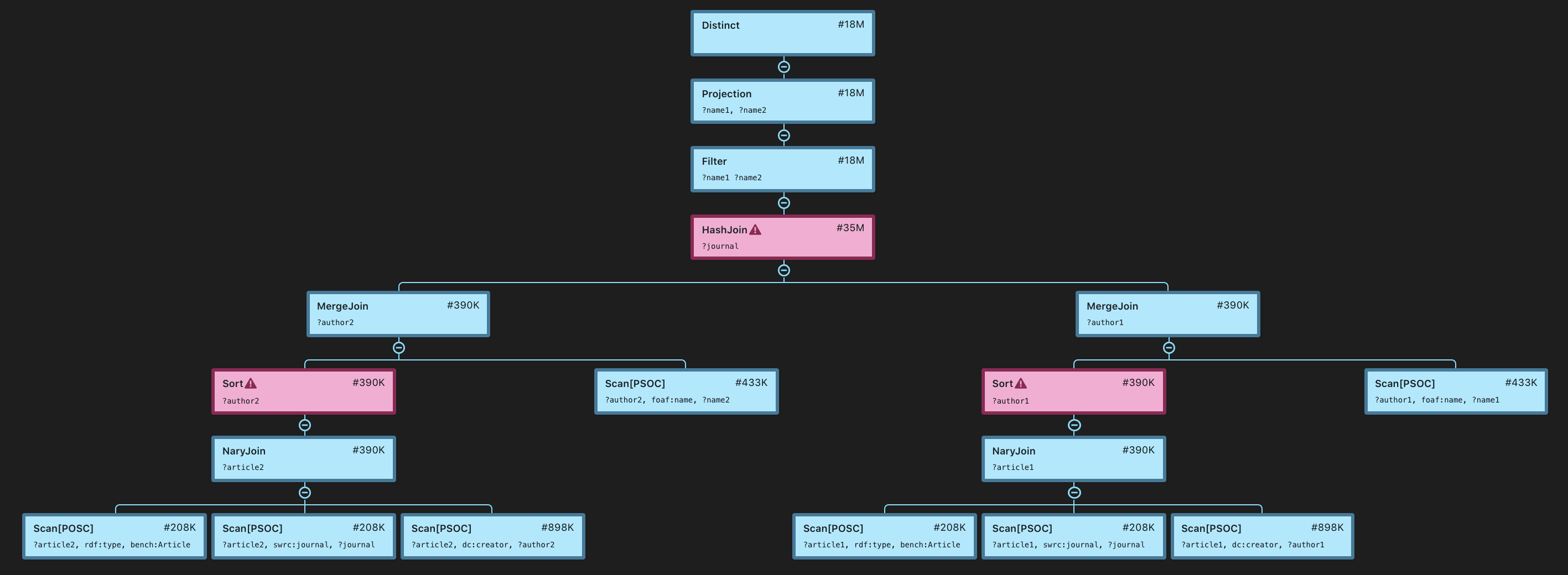
The query returns all distinct pairs of authors who published (possibly different) articles in the same journal. It returns more than 18M results from a database of 5M triples. Here’s the plan:
Distinct [#17.7M]
`─ Projection(?name1, ?name2) [#17.7M]
   `─ Filter(?name1 < ?name2) [#17.7M]
      `─ HashJoin(?journal) [#35.4M]
         +─ MergeJoin(?author2) [#390K]
         │  +─ Sort(?author2) [#390K]
         │  │  `─ NaryJoin(?article2) [#390K]
         │  │     +─ Scan[POSC](?article2, rdf:type, bench:Article) [#208K]
         │  │     +─ Scan[PSOC](?article2, swrc:journal, ?journal) [#208K]
         │  │     `─ Scan[PSOC](?article2, dc:creator, ?author2) [#898K]
         │  `─ Scan[PSOC](?author2, foaf:name, ?name2) [#433K]
         `─ MergeJoin(?author1) [#390K]
            +─ Sort(?author1) [#390K]
            │  `─ NaryJoin(?article1) [#390K]
            │     +─ Scan[POSC](?article1, rdf:type, bench:Article) [#208K]
            │     +─ Scan[PSOC](?article1, swrc:journal, ?journal) [#208K]
            │     `─ Scan[PSOC](?article1, dc:creator, ?author1) [#898K]
            `─ Scan[PSOC](?author1, foaf:name, ?name1) [#433K]

This query requires an expensive join on ?journal which is evident from the plan (it’s a hash join in this case). It produces more than 18M results (Stardog expects 17.7M which is fairly accurate in this case) that need to be filtered and examined for duplicates. Given all this information from the plan, the only reasonable way to address the problem would be to restrict the criteria, e.g. to particular journals, people, time periods, etc.
If a query is well-formulated and selective, but performance is unsatisfactory, one may look closer at the pipeline breakers, e.g. this part of the query 5b plan:
MergeJoin(?person) [#391K]
+─ Sort(?person) [#391K]
|  `─ MergeJoin(?article) [#391K]
|     +─ Scan[POSC](?article, rdf:type, bench:Article) [#208K]
|     `─ Scan[PSOC](?article, dc:creator, ?person) [#898K]
`─ Scan[PSOC](?person, foaf:name, ?name) [#433K]
A reasonable thing to do would be to evaluate the join of ?article rdf:type bench:Article and ?article dc:creator ?person separately, i.e. as a separate queries, to see if the estimation of 391K is reasonably accurate and to get an idea about memory pressure. This is a valuable piece of information for a performance problem report, especially when the data cannot be shared with us. Similar analysis can be done for hash joins.
In addition to pipeline breakers, there could be other clear indicators of performance problems. One of them is the presence of LoopJoin nodes in the plan. Stardog performs the nested loop join algorithm which evaluates the join by going through the Cartesian product of its inputs. This is the slowest join algorithm and it is used only as a last resort. It sometimes, but not always, indicates a problem with the query. One example is the query 5a in SP2B:
 SELECT DISTINCT ?person ?name
 WHERE {
   ?article rdf:type bench:Article .
   ?article dc:creator ?person .
   ?inproc rdf:type bench:Inproceedings .
   ?inproc dc:creator ?person2 .
   ?person foaf:name ?name .
   ?person2 foaf:name ?name2
   FILTER (?name=?name2)
 }
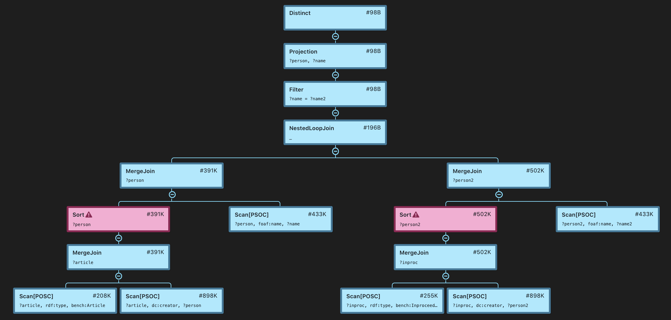
The query is very similar to query 5b at the top but runs much slower. The plan shows why:
Distinct [#98066.0M]
`─ Projection(?person, ?name) [#98066.0M]
   `─ Filter(?name = ?name2) [#98066.0M]
      `─ NestedLoopJoin(_) [#196132.0M]
         +─ MergeJoin(?person) [#391K]
         │  +─ Sort(?person) [#391K]
         │  │  `─ MergeJoin(?article) [#391K]
         │  │     +─ Scan[POSC](?article, rdf:type, bench:Article) [#208K]
         │  │     `─ Scan[PSOC](?article, dc:creator, ?person) [#898K]
         │  `─ Scan[PSOC](?person, foaf:name, ?name) [#433K]
         `─ MergeJoin(?person2) [#502K]
            +─ Sort(?person2) [#502K]
            │  `─ MergeJoin(?inproc) [#502K]
            │     +─ Scan[POSC](?inproc, rdf:type, bench:Inproceedings) [#255K]
            │     `─ Scan[PSOC](?inproc, dc:creator, ?person2) [#898K]
            `─ Scan[PSOC](?person2, foaf:name, ?name2) [#433K]

The loop join near the top of the plan computes the Cartesian product of the arguments which produces almost 200B solutions. This is because there is no shared variable between the parts of the query which correspond to authors of articles and conference proceedings papers, respectively. The filter condition ?name = ?name2 cannot be transformed into an equi-join because the semantics of term equality used in filters is different from the solution compatibility semantics used for checking join conditions.
The difference manifests itself in the presence of numerical literals, e.g. "1"^^xsd:integer = "1.0"^^xsd:float, where they are different RDF terms. However, as long as all names in the data are strings, one can re-formulate this query by renaming ?name2 to ?name which would enable Stardog to use a more efficient join algorithm.
Learning how to read Stardog query plans not only gives you insight into how it’s handling your queries against your data but will also prepare you to use the upcoming query hints capability to tune Stardog for maximum performance.