Optimization
This page describes factors that affect Virtual Graph query performance.
Page Contents
Overview
There are many choices to make when setting up a data source and virtual graph. Many of these choices can affect how a query over that virtual graph will perform. This page describes how data source options and virtual graph mappings can affect the efficiency of those queries.
In almost all cases, the goal will be to minimize the number of joins and unions in the query plan. An introduction to query plans can be found here. The examples in this section can be found in the stardog-examples GitHub repository.
Unique Keys
Stardog uses information on unique columns from table metadata to reduce the number of joins in the queries it generates. To illustrate the significance of unique columns in a table, consider the following table and virtual graph mapping:
CREATE TABLE Bands(id INTEGER, -- note no primary key
                   name VARCHAR(20),
                   country VARCHAR(20),
                   year_formed int);

INSERT INTO Bands VALUES(1, 'Aerosmith', 'USA', 1970);
INSERT INTO Bands VALUES(1, 'Errorsmith', 'USA', 2022);
PREFIX : <urn:>

MAPPING :uniques
FROM SQL {
  SELECT * FROM Bands
}
TO {
  ?band a :Band ;
    rdfs:label ?name ;
    :country ?country ;
    :yearFormed ?year_formed .
}
WHERE {
  BIND(TEMPLATE("urn:band:{id}") AS ?band)
}
This leads to a graph with a single node and two values for each of two properties; rdfs:label and :yearFormed:
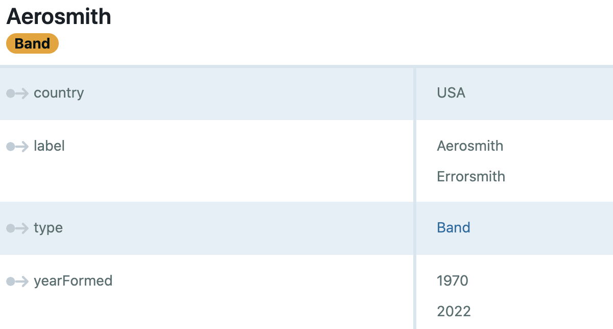
Because of the way this node is mapped, the association between the label and year that existed in the table is lost. (See Mapping Denormalized Data for a mapping that retains the relationship.) A query that matches both the label and year must return the cross product of the two solutions for the two triple patterns:
SELECT * FROM <virtual://uniques> {
    ?s rdfs:label ?label ;
       :yearFormed ?yearFormed .
}
+--------+--------------+------------+
|   s    |    label     | yearFormed |
+--------+--------------+------------+
| band:1 | "Aerosmith"  | "1970"     |
| band:1 | "Aerosmith"  | "2022"     |
| band:1 | "Errorsmith" | "1970"     |
| band:1 | "Errorsmith" | "2022"     |
+--------+--------------+------------+
In keeping with Stardog’s principle to “move the compute to the data”, the join is pushed down to the SQL:
SELECT "Bands"."id", "Bands"."name", "Bands0"."year_formed" AS "year_formed0"
FROM "Bands"
INNER JOIN "Bands" AS "Bands0"
ON "Bands"."id" = "Bands0"."id"
This join is necessary to ensure correct results whenever the join variable (?s in the last example) is bound to a TEMPLATE that’s built from a set of columns that are not known to be unique in the backing table. In this example, the TEMPLATE is built from the single column id:
BIND(TEMPLATE("urn:band:{id}") AS ?band)
Suppose our table did not contain multiple rows for a given id:
DELETE FROM Bands WHERE id=1 AND year_formed=2022
The query would return a single row, yet the plan continues to contain the join:
SELECT * FROM <virtual://uniques> {
    ?s rdfs:label ?label ;
       :yearFormed ?yearFormed .
}
From <virtual://uniques>
VirtualGraphSql<virtual://uniques> [#1] {
   RelNode=
      LogicalProject(id=[$0], year_formed=[$3], name0=[$5])
        LogicalJoin(condition=[AND(=($0, $4), IS NOT NULL($3), IS NOT NULL($5))], joinType=[inner])
          JdbcTableScan(table=[[examples, Bands]])
          JdbcTableScan(table=[[examples, Bands]])
   Query=
      SELECT `Bands`.`id`, `Bands`.`year_formed`, `Bands0`.`name` `name0`
      FROM `examples`.`Bands`
      INNER JOIN `examples`.`Bands` `Bands0` ON `Bands`.`id` = `Bands0`.`id` AND `Bands`.`year_formed` IS NOT NULL AND `Bands0`.`name` IS NOT NULL
   Vars=
      ?s <- TEMPLATE(urn:band:{id/0})
      ?label <- COLUMN($2)^^xsd:string
      ?yearFormed <- COLUMN($1)^^xsd:string
} [#1]
+--------+-------------+------------+
|   s    |    label    | yearFormed |
+--------+-------------+------------+
| band:1 | "Aerosmith" | "1970"     |
+--------+-------------+------------+
If the id column is unique, then that join is no longer necessary. Stardog examines the metadata of the backing table and recognizes any primary or unique keys that are defined as constraints in the table’s DDL. However, many data sources, in particular big data architectures such as Databricks, Hive, MongoDB, and Athena, do not support these constraints. For such platforms, we can indicate column uniqueness (even if not enforced by the database) with the unique.key.sets data source configuration option, leading to a SQL query with no join:
unique.key.sets=(Bands.id)
SELECT `id`, `name`, `year_formed`
FROM `listeners`.`Bands`
WHERE `year_formed` IS NOT NULL
The unique.key.sets property can be used with all database types, not just those that do not support key constraints. For databases that have key constraints defined, Stardog will combine the database constraints and the keys set in the unique.key.sets property.
Supplement a table’s DDL-defined constraints with the unique.key.sets property for any sets of fields that comprise a unique key.
Denormalized Data
Another potential cause of inefficient queries is mapping to denormalized tables. In the last example, the table was mapped in a way that lost the association between the band name and its year formed. Now we’ll consider an example where we’ll seek to retain such a relationship.
We’ll use this table:
CREATE TABLE Roles(movie_id  INTEGER     NOT NULL,
                   title     VARCHAR(20) NOT NULL,
                   year      VARCHAR(20) NOT NULL,
                   actor_id  INTEGER     NOT NULL,
                   name      VARCHAR(20) NOT NULL,
                   char_name VARCHAR(20) NOT NULL,
                   PRIMARY KEY (movie_id, actor_id));

INSERT INTO Roles VALUES(1, 'The Princess Bride', 1987, 1, 'Robin Wright',      'Buttercup');
INSERT INTO Roles VALUES(2, 'Unbreakable',        2000, 1, 'Robin Wright Penn', 'Audrey Dunn');
INSERT INTO Roles VALUES(3, 'Apocalypse Now',     1979, 3, 'Larry Fishburne',   'Mr. Clean');
INSERT INTO Roles VALUES(4, 'The Matrix',         1999, 3, 'Laurence Fishburne','Morpheus');
The purpose of the Roles table in this example is to link Movies and Actors. In a normalized database, we expect the name of an actor to be a column of an Actors table; however, in this example, the actor’s name is in the Roles table. An inspection of the data reveals that, unlike the result of a join of two normalized Movies and Actors tables, the actor’s name is not always the same. So while this table is denormalized, in the sense that title and year could have come from a normalized Movie table, we would not see this variation in the actor’s name in a normalized table. We can think of the name field as representing a creditedAs relationship – the name the actor had at the time the movie was released.
This mapping, which treats the Roles table as a source of truth for :Actor nodes, can lead to inefficient query plans:
PREFIX : <urn:>

MAPPING :denormalized1
FROM SQL {
  SELECT * FROM Roles
}
TO {
  ?movie a :Movie ;
    rdfs:label ?title ;
    :releaseYear "?year"^^xsd:integer ;
    :actor ?actor .

  ?actor a :Actor ;
    rdfs:label ?name .
}
WHERE {
  BIND(TEMPLATE("urn:movie:{movie_id}") AS ?movie)
  BIND(TEMPLATE("urn:actor:{actor_id}") AS ?actor)
}
With such a mapping, what should we expect from a simple query for an actor’s name?
SELECT * FROM <virtual://denormalized1> {
    ?s a :Actor ;
       rdfs:label ?name .
}
+-------------+----------------------+
|      s      |         name         |
+-------------+----------------------+
| urn:actor:1 | "Robin Wright Penn"  |
| urn:actor:1 | "Robin Wright"       |
| urn:actor:3 | "Larry Fishburne"    |
| urn:actor:3 | "Laurence Fishburne" |
+-------------+----------------------+
From <virtual://denormalized1>
VirtualGraphSql<virtual://denormalized1> [#1] {
   RelNode=
      LogicalProject(actor_id=[$3], name=[$4])
        JdbcTableScan(table=[[examples, Roles]])
   Query=
      SELECT `actor_id`, `name`
      FROM `examples`.`Roles`
   Vars=
      ?s <- TEMPLATE(urn:actor:{actor_id/0})
      ?name <- COLUMN($1)^^xsd:string
} [#1]
In this scenario, we should recognize that the Actor name does not belong to the actor, but rather to the relationship between the actor and the movie. For this example, we’ll model that by promoting the actor/movie relationship to its own Role node. The mapping looks like this:
PREFIX : <urn:>

MAPPING :denormalized2
FROM SQL {
  SELECT * FROM Roles
}
TO {
  ?movie a :Movie ;
    rdfs:label ?title ;
    :releaseYear "?year"^^xsd:integer .

  ?role a :Role ;
    :movie ?movie ;
    :character ?char_name ;
    :actor ?actor ;
    :creditedAs ?name .
}
WHERE {
  BIND(TEMPLATE("urn:role:{movie_id}_{actor_id}") AS ?role)
  BIND(TEMPLATE("urn:movie:{movie_id}") AS ?movie)
  BIND(TEMPLATE("urn:actor:{actor_id}") AS ?actor)
}
The query becomes:
SELECT * FROM <virtual://denormalized2> {
    [] a :Role ;
        :actor ?actor ;
        :creditedAs ?name .
}
From <virtual://denormalized2>
VirtualGraphSql<virtual://denormalized2> [#1] {
   RelNode=
      LogicalProject(actor_id=[$3], name=[$4])
        JdbcTableScan(table=[[examples, Roles]])
   Query=
      SELECT `actor_id`, `name`
      FROM `examples`.`Roles`
   Vars=
      ?actor <- TEMPLATE(urn:actor:{actor_id/0})
      ?name <- COLUMN($1)^^xsd:string
} [#1]
The query still returns two names for the same actor:
+-------------+----------------------+
|    actor    |         name         |
+-------------+----------------------+
| urn:actor:1 | "Robin Wright Penn"  |
| urn:actor:1 | "Robin Wright"       |
| urn:actor:3 | "Larry Fishburne"    |
| urn:actor:3 | "Laurence Fishburne" |
+-------------+----------------------+
Ideally, there is another Actors table that contains the actor’s preferred name. Unfortunately, we’re often in a position where all we have access to is denormalized data in a data lake or warehouse despite the data existing in normalized form elsewhere in the enterprise. This needs to change. If possible, include the normalized tables in the lake or warehouse as well.
When you have no alternative, you may be tempted to create a mapping that uses a SQL query to renormalize the table:
PREFIX : <urn:>

MAPPING :antipattern
FROM SQL {
  SELECT t1.actor_id AS id, name
  FROM Roles AS t1
  JOIN (
    -- "year" is a reserved word in Stardog's parser so quoting
    -- Use the native identifier quote character for your platform or
    -- include parser.sql.quoting=ANSI as a VG property to use double quotes
    SELECT actor_id, max("year") AS maxyear
    FROM Roles
    GROUP BY actor_id) AS t2
  ON t1.actor_id = t2.actor_id AND t1."year" = t2.maxyear
}
TO {
  ?actor a :Actor ;
    rdfs:label ?name .
}
WHERE {
  BIND(TEMPLATE("urn:actor:{id}") AS ?actor)
}
This works in a pinch (assuming actors do not have multiple roles in a year), but it leads to inefficient plans:
SELECT * FROM <virtual://denormalized2> {
    ?s a :Actor ;
       rdfs:label ?name .
}
From <virtual://denormalized2>
VirtualGraphSql<virtual://denormalized2> [#1] {
   RelNode=
      LogicalProject(actor_id=[$3], name=[$4])
        LogicalJoin(condition=[AND(=($2, $7), =($3, $6))], joinType=[inner])
          JdbcTableScan(table=[[examples, Roles]])
          LogicalAggregate(group=[{0}], maxyear=[MAX($1)])
            LogicalProject(actor_id=[$3], year=[$2])
              JdbcTableScan(table=[[examples, Roles]])
   Query=
      SELECT `Roles`.`actor_id`, `Roles`.`name`
      FROM `examples`.`Roles`
      INNER JOIN (SELECT `actor_id`, MAX(`year`) `maxyear`
      FROM `examples`.`Roles` `Roles0`
      GROUP BY `actor_id`) `t0` ON `Roles`.`year` = `t0`.`maxyear` AND `Roles`.`actor_id` = `t0`.`actor_id`
   Vars=
      ?s <- TEMPLATE(urn:actor:{id/0})
      ?name <- COLUMN($1)^^xsd:string
} [#1]
+-------------+----------------------+
|      s      |         name         |
+-------------+----------------------+
| urn:actor:1 | "Robin Wright Penn"  |
| urn:actor:3 | "Laurence Fishburne" |
+-------------+----------------------+
If you know that actors always have the same name, you can use an aggregation to select a single name per Actor. Note the use of the relatively new ANY_VALUE aggregate function. If your platform doesn’t support ANY_VALUE, you can use the more common (but less efficient) MIN or MAX functions.
MAPPING :renormalizing_by_aggregated_name
FROM SQL {
  SELECT actor_id AS id, ANY_VALUE(name) as name
  FROM Roles
  GROUP BY actor_id
}
TO {
  ?actor a :Actor ;
    rdfs:label ?name .
}
WHERE {
  BIND(TEMPLATE("urn:actor:{id}") AS ?actor)
}
A GROUP BY has the effect of creating a relation (table) with the group by terms serving as a unique key. As of version 11.2, self joins on group by columns are eliminated:
SELECT * FROM <virtual://denormalized3> {
    ?s a :Actor ;
       rdfs:label ?name .
}
From <virtual://denormalized3>
VirtualGraphSql<virtual://denormalized3> [#1] {
   RelNode=
      LogicalAggregate(group=[{0}], name=[ANY_VALUE($1)])
        LogicalProject(actor_id=[$3], name=[$4])
          JdbcTableScan(table=[[examples, Roles]])
   Query=
      SELECT `actor_id`, ANY_VALUE(`name`) `name`
      FROM `examples`.`Roles`
      GROUP BY `actor_id`
   Vars=
      ?s <- TEMPLATE(urn:actor:{id/0})
      ?name <- COLUMN($1)^^xsd:string
} [#1]
In general, if you have mappings like this, it’s good to consider materializing the results to a Stardog database or creating a cache for the virtual graph.
When mapping to a denormalized table, create a node mapped to a template built with the keys of the row and treat the non-key columns as properties of that node. Resist the urge to treat denormalized tables as an authoritative source of nodes with IRIs built from non-key fields. See the next section, Map rdf:type Conservatively, for a deeper exploration of the authoritative source of truth for nodes.
See this blog post for a more detailed discussion of mapping denormalized data.
Map rdf:type Conservatively
Notice in the last example that there was no mapping for rdf:type :Actor. This is because of an assumption that there is another mapping to a normalized Actors table:
CREATE TABLE Actors(id   INTEGER     NOT NULL,
                    name VARCHAR(20) NOT NULL,
                    PRIMARY KEY (id));

INSERT INTO Actors VALUES(1, 'Robin Wright');
INSERT INTO Actors VALUES(2, 'Tom Hanks');
INSERT INTO Actors VALUES(3, 'Laurence Fishburne');
First, let’s create a mappings file where the ?actor a :Actor triple pattern is defined in both the Roles and Actors mappings:
PREFIX : <urn:>

MAPPING :actor1_actors
FROM SQL {
  SELECT * FROM Actors
}
TO {
  ?actor a :Actor ;
    rdfs:label ?name .
}
WHERE {
  BIND(TEMPLATE("urn:actor:{id}") AS ?actor)
}

;

MAPPING :actors1_roles
FROM SQL {
  SELECT * FROM Roles
}
TO {
  ?movie a :Movie ;
    rdfs:label ?title ;
    :releaseYear "?year"^^xsd:integer .

  ?role a :Role ;
    :movie ?movie ;
    :character ?char_name ;
    :actor ?actor ;
    :creditedAs ?name .

  # Do we really want the Roles table to be an authoritative source for Actors?
  ?actor a :Actor .
}
WHERE {
  BIND(TEMPLATE("urn:role:{movie_id}_{actor_id}") AS ?role)
  BIND(TEMPLATE("urn:movie:{movie_id}") AS ?movie)
  BIND(TEMPLATE("urn:actor:{actor_id}") AS ?actor)
}
Do we get the expected result from a simple get-all-Actors query?
SELECT * FROM <virtual://actors1> {
    ?s a :Actor
}
+-------------+
|      s      |
+-------------+
| urn:actor:3 |
| urn:actor:1 |
| urn:actor:2 |
| urn:actor:1 |
| urn:actor:1 |
| urn:actor:3 |
| urn:actor:3 |
+-------------+
Let’s look at the plan:
From <virtual://actors1>
VirtualGraphSql<virtual://actors1> [#2] {
   RelNode=
      LogicalUnion(all=[true])
        LogicalProject(id=[$0])
          JdbcTableScan(table=[[examples, Actors]])
        LogicalProject(id=[$3])
          JdbcTableScan(table=[[examples, Roles]])
   Query=
      SELECT `id`
      FROM `examples`.`Actors`
      UNION ALL
      SELECT `actor_id` `id`
      FROM `examples`.`Roles`
   Vars=
      ?s <- TEMPLATE(urn:actor:{id/0})
} [#2]
The plan indicates a UNION of two virtual graphs. The first returns the actors defined by the Actors table, and the second returns the actors referenced in the Movies table.
Is this correct? To answer, we need to think in terms of meaning, authority, and redundancy. In our model, what is the source of truth for who is an Actor? If an actor appears in the Movies table but not in the Actors table, is it still an Actor? If the answer is ‘no’, we should not include the ?actor rdf:type :Actor triple pattern in the mapping. Removing it eliminates the duplicate results and simplifies the query plan:
+-------------+
|      s      |
+-------------+
| urn:actor:3 |
| urn:actor:1 |
| urn:actor:2 |
+-------------+
From <virtual://actors2>
VirtualGraphSql<virtual://actors2> [#1] {
   RelNode=
      LogicalProject(id=[$0])
        JdbcTableScan(table=[[examples, Actors]])
   Query=
      SELECT `id`
      FROM `examples`.`Actors`
   Vars=
      ?s <- TEMPLATE(urn:actor:{id/0})
} [#1]
Reserve rdf:type in mappings for those sources that represent the authoritative source of truth on which IRIs are what type.
Unique Predicates
In the last example, we explored a case where we were able to eliminate a UNION with careful mapping. This and the following example illustrate other cases where avoidable UNIONS can be introduced. If we’re not careful, these various causes can combine with each other leading to a combinatorial explosion of UNIONS.
A common predicate (the middle term of an RDF triple) is rdfs:label. It’s handy because client applications like Stardog Explorer have built-in knowledge of this predicate, so we dutifully include a mapping to rdfs:label for every node we map.
The drawback to a common predicate is it is no longer selective. If all nodes have the same predicate, a query that attempts to match nodes with a particular value for that predicate will need to check all possible node types for that value.
Consider these tables and mapping:
CREATE TABLE Movies(id    INTEGER     NOT NULL,
                    title VARCHAR(20) NOT NULL,
                    year  VARCHAR(20) NOT NULL,
                    PRIMARY KEY (id));

INSERT INTO Movies VALUES(1, 'The Princess Bride', 1987);
INSERT INTO Movies VALUES(2, 'Unbreakable',        2000);
INSERT INTO Movies VALUES(3, 'Forest Gump',        1994);

CREATE TABLE Actors(id   INTEGER     NOT NULL,
                    name VARCHAR(20) NOT NULL,
                    PRIMARY KEY (id));

INSERT INTO Actors VALUES(1, 'Robin Wright');
INSERT INTO Actors VALUES(2, 'Tom Hanks');
PREFIX : <urn:>

MAPPING :predicates-actors
FROM SQL {
  SELECT * FROM Actors
}
TO {
  ?actor a :Actor ;
    :name ?name ;
    rdfs:label ?name .
}
WHERE {
  BIND(TEMPLATE("urn:actor:{id}") AS ?actor)
}

;

MAPPING :predicates-movies
FROM SQL {
  SELECT * FROM Movies
}
TO {
  ?movie a :Movie ;
    :title ?title ;
    rdfs:label ?title ;
    :releaseYear "?year"^^xsd:integer .
}
WHERE {
  BIND(TEMPLATE("urn:movie:{id}") AS ?movie)
}
A query to find the node with the rdfs:label “Tom Hanks” has to search both Actors and Movies.
SELECT * {
    GRAPH <virtual://predicates> {
        ?s rdfs:label "Tom Hanks"
    }
}
VirtualGraphSql<virtual://predicates> [#2] {
   RelNode=
      LogicalUnion(all=[true])
        LogicalProject(TYPE_1=[126], VAL_1=[||('urn:actor:', CAST($0):VARCHAR(2048) NOT NULL)])
          LogicalFilter(condition=[=($1, 'Tom Hanks')])
            JdbcTableScan(table=[[examples, Actors]])
        LogicalProject(TYPE_1=[126], VAL_1=[||('urn:movie:', CAST($0):VARCHAR(2048) NOT NULL)])
          LogicalFilter(condition=[=($1, 'Tom Hanks')])
            JdbcTableScan(table=[[examples, Movies]])
   Query=
      SELECT 126 `TYPE_1`, CONCAT('urn:actor:', CAST(`id` AS VARCHAR(2048))) `VAL_1`
      FROM `examples`.`Actors`
      WHERE `name` = 'Tom Hanks'
      UNION ALL
      SELECT 126 `TYPE_1`, CONCAT('urn:movie:', CAST(`id` AS VARCHAR(2048))) `VAL_1`
      FROM `examples`.`Movies`
      WHERE `title` = 'Tom Hanks'
   Vars=
      ?s <- VARTYPE(type={$0}, value={$1})
} [#2]
A query on the more selective :name predicate needs to search only the Actors table:
SELECT * {
    GRAPH <virtual://predicates> {
        ?s :name "Tom Hanks"
    }
}
VirtualGraphSql<virtual://predicates> [#1] {
   RelNode=
      LogicalProject(id=[$0])
        LogicalFilter(condition=[=($1, 'Tom Hanks')])
          JdbcTableScan(table=[[examples, Actors]])
   Query=
      SELECT `id`
      FROM `examples`.`Actors`
      WHERE `name` = 'Tom Hanks'
   Vars=
      ?s <- TEMPLATE(urn:actor:{id/0})
} [#1]
When writing queries, favor selective predicates over common predicates.
Query rdf:type Liberally
If a more selective predicate is not available, adding constraints to the query can also make it more efficient. The following query adds the constraint that the result must be an :Actor, which eliminates the UNION from the plan as well:
SELECT * {
    GRAPH <virtual://predicates> {
        ?s a :Actor ;
           rdfs:label "Tom Hanks" .
    }
}
VirtualGraphSql<virtual://predicates> [#1] {
   RelNode=
      LogicalProject(id=[$0])
        LogicalFilter(condition=[=($1, 'Tom Hanks')])
          JdbcTableScan(table=[[examples, Actors]])
   Query=
      SELECT `id`
      FROM `examples`.`Actors`
      WHERE `name` = 'Tom Hanks'
   Vars=
      ?s <- TEMPLATE(urn:actor:{id/0})
} [#1]
In addition to using selective predicates, adding triple patterns with constant properties can make a query more selective.
Mutually Exclusive Templates
In the last example, we had a query that scanned two tables because it was matching a predicate that appeared in the mappings for both tables. We resolved it by matching on a more selective predicate, but we also saw that we could change the query to include a triple pattern to select the nodes of type :Actor. Recall the query:
SELECT * {
    GRAPH <virtual://predicates> {
        ?s a :Actor .
        ?s rdfs:label "Tom Hanks" .
    }
}
VirtualGraphSql<virtual://predicates> [#1] {
   RelNode=
      LogicalProject(id=[$0])
        LogicalFilter(condition=[=($1, 'Tom Hanks')])
          JdbcTableScan(table=[[examples, Actors]])
   Query=
      SELECT `id`
      FROM `examples`.`Actors`
      WHERE `name` = 'Tom Hanks'
   Vars=
      ?s <- TEMPLATE(urn:actor:{id/0})
} [#1]
This worked because Stardog was able to rule out the Movies table because its id field is mapped to an IRI with an urn:movie: prefix while the ?s a :Actor triple pattern matched only IRIs that have a urn:actor: prefix. Since no IRI can begin with both strings, Stardog eliminated the UNION to the Actors table.
If the :Actor and :Movie IRIs were mapped to templates with a common prefix, things would be different:
PREFIX : <urn:>

MAPPING :templates-actors
FROM SQL {
  SELECT * FROM Actors
}
TO {
  ?actor a :Actor ;
    :name ?name ;
    rdfs:label ?name .
}
WHERE {
  BIND(TEMPLATE("urn:node:{id}") AS ?actor)
}

;

MAPPING :templates-movies
FROM SQL {
  SELECT * FROM Movies
}
TO {
  ?movie a :Movie ;
    :title ?title ;
    rdfs:label ?title ;
    :releaseYear "?year"^^xsd:integer .
}
WHERE {
  BIND(TEMPLATE("urn:node:{id}") AS ?movie)
}
SELECT * {
    GRAPH <virtual://templates> {
        ?s a :Actor .
        ?s rdfs:label "Tom Hanks" .
    }
}
VirtualGraphSql<virtual://templates> [#2] {
   RelNode=
      LogicalUnion(all=[true])
        LogicalProject(id=[$0])
          LogicalFilter(condition=[=($1, 'Tom Hanks')])
            JdbcTableScan(table=[[examples, Actors]])
        LogicalProject(id=[$0])
          LogicalJoin(condition=[AND(=($0, $3), =($1, 'Tom Hanks'))], joinType=[inner])
            JdbcTableScan(table=[[examples, Movies]])
            JdbcTableScan(table=[[examples, Actors]])
   Query=
      SELECT `id`
      FROM `examples`.`Actors`
      WHERE `name` = 'Tom Hanks'
      UNION ALL
      SELECT `Movies`.`id`
      FROM `examples`.`Movies`
      INNER JOIN `examples`.`Actors` `Actors0` ON `Movies`.`id` = `Actors0`.`id` AND `Movies`.`title` = 'Tom Hanks'
   Vars=
      ?s <- TEMPLATE(urn:node:{id/0})
} [#2]
For two mappings to be mutually exclusive, they must contain conflicting text in either their prefix or suffix. A template urn:{big} could match urn:actor:{small}:imdb if, say, big contained actor:1:imdb and small contained 1. In a simple query, Stardog will refuse to match these as a performance optimization. However, in the case of service joins (where we join data from two different virtual graphs), or in cases where we join local (materialized) data with virtual data, Stardog cannot avoid attempting that match.
If two tables should not create the same IRI, do not rely on the mapped columns having non-overlapping values. Create mutually exclusive templates so that Stardog can know that these IRIs are guaranteed not to match.
Query Inputs and Outputs
In the Unique Predicates section, we explored how querying for nodes with an unselective predicate such as rdfs:label can lead to poor performance. However, we also have a requirement to have an rdfs:label mapping for client tools like Stardog Explorer. How do we satisfy both needs? The key is to think in terms of virtual graph inputs and outputs.
Going back to the tables and mappings from the Unique Predicates section:
CREATE TABLE Movies(id    INTEGER     NOT NULL,
                    title VARCHAR(20) NOT NULL,
                    year  VARCHAR(20) NOT NULL,
                    PRIMARY KEY (id));

INSERT INTO Movies VALUES(1, 'The Princess Bride', 1987);
INSERT INTO Movies VALUES(2, 'Unbreakable',        2000);
INSERT INTO Movies VALUES(3, 'Forest Gump',        1994);

CREATE TABLE Actors(id   INTEGER     NOT NULL,
                    name VARCHAR(20) NOT NULL,
                    PRIMARY KEY (id));

INSERT INTO Actors VALUES(1, 'Robin Wright');
INSERT INTO Actors VALUES(2, 'Tom Hanks');
PREFIX : <urn:>

MAPPING :predicates-actors
FROM SQL {
  SELECT * FROM Actors
}
TO {
  ?actor a :Actor ;
    :name ?name ;
    rdfs:label ?name .
}
WHERE {
  BIND(TEMPLATE("urn:actor:{id}") AS ?actor)
}

;

MAPPING :predicates-movies
FROM SQL {
  SELECT * FROM Movies
}
TO {
  ?movie a :Movie ;
    :title ?title ;
    rdfs:label ?title ;
    :releaseYear "?year"^^xsd:integer .
}
WHERE {
  BIND(TEMPLATE("urn:movie:{id}") AS ?movie)
}
Recall the query from that section:
SELECT * {
    GRAPH <virtual://predicates> {
        ?s rdfs:label "Tom Hanks"
    }
}
For this query, the plan was:
VirtualGraphSql<virtual://predicates> [#2] {
   RelNode=
      LogicalUnion(all=[true])
        LogicalProject(TYPE_1=[126], VAL_1=[||('urn:actor:', CAST($0):VARCHAR(2048) NOT NULL)])
          LogicalFilter(condition=[=($1, 'Tom Hanks')])
            JdbcTableScan(table=[[examples, Actors]])
        LogicalProject(TYPE_1=[126], VAL_1=[||('urn:movie:', CAST($0):VARCHAR(2048) NOT NULL)])
          LogicalFilter(condition=[=($1, 'Tom Hanks')])
            JdbcTableScan(table=[[examples, Movies]])
   Query=
      SELECT 126 `TYPE_1`, CONCAT('urn:actor:', CAST(`id` AS VARCHAR(2048))) `VAL_1`
      FROM `examples`.`Actors`
      WHERE `name` = 'Tom Hanks'
      UNION ALL
      SELECT 126 `TYPE_1`, CONCAT('urn:movie:', CAST(`id` AS VARCHAR(2048))) `VAL_1`
      FROM `examples`.`Movies`
      WHERE `title` = 'Tom Hanks'
   Vars=
      ?s <- VARTYPE(type={$0}, value={$1})
} [#2]
There is one SQL query for each mapping of the rdfs:label predicate (those mappings are the triple patterns ?movie rdfs:label ?title and ?actor rdfs:label ?name). For each of those triple patterns, the constant Tom Hanks was bound to the object of the triple pattern, while the subject was bound to the variable ?s.
In this example, the constant Tom Hanks is an input, and the variable ?s is an output. Stardog must look in every table that maps the object of an rdfs:label triple pattern to a variable and constrain that variable to the constant:
SELECT `id`
FROM `examples`.`Actors`
WHERE `name` = 'Tom Hanks'
And:
SELECT `id`
FROM `examples`.`Movies`
WHERE `title` = 'Tom Hanks'
This can be inefficient if we only want actors, so in the prior example we queried on the more selective :name instead of the more general rdfs:label:
SELECT * {
    GRAPH <virtual://predicates> {
        ?s :name "Tom Hanks"
    }
}
If we need rdfs:label, we bind its object to a variable while binding the object of :name to a constant:
SELECT * {
    GRAPH <virtual://predicates> {
        ?s :name "Tom Hanks" ;
            rdfs:label ?label .
    }
}
Because we’re looking up the subject ?s by :name, we avoid the UNION in the plan:
VirtualGraphSql<virtual://predicates> [#1] {
   RelNode=
      LogicalFilter(condition=[=($1, 'Tom Hanks')])
        JdbcTableScan(table=[[examples, Actors]])
   Query=
      SELECT *
      FROM `examples`.`Actors`
      WHERE `name` = 'Tom Hanks'
   Vars=
      ?s <- TEMPLATE(urn:actor:{id/0})
      ?label <- COLUMN($1)^^xsd:string
} [#1]
When writing queries, whenever possible, bind constants to selective or unique properties (making them inputs to the virtual graph) and variables to properties that are common to many node types (making those variables outputs).
SQL Functions and Query Outputs
Suppose we would like to compose an rdfs:label by combining multiple fields. It is common for movies to be remade and released with the same title. A nice way to tell them apart would be to include the year of release in the label. Such a field can be created using an expression in the SQL query:
CREATE TABLE Remakes(id INTEGER,
                     title        VARCHAR(40) NOT NULL,
                     release_year INTEGER     NOT NULL,
                     PRIMARY KEY (id),
                     KEY (title, release_year));

INSERT INTO Remakes VALUES(1, '3:10 to Yuma', 1957);
INSERT INTO Remakes VALUES(2, '3:10 to Yuma', 2007);
INSERT INTO Remakes VALUES(3, 'A Star Is Born', 1937);
INSERT INTO Remakes VALUES(4, 'A Star Is Born', 1976);
INSERT INTO Remakes VALUES(5, 'A Star Is Born', 2018);
INSERT INTO Remakes VALUES(6, 'Ocean''s Eleven', 1960);
INSERT INTO Remakes VALUES(7, 'Ocean''s Eleven', 2001);
INSERT INTO Remakes VALUES(8, 'True Grit', 1969);
INSERT INTO Remakes VALUES(9, 'True Grit', 2010);
PREFIX : <urn:>

MAPPING :remakes
FROM SQL {
  -- Mixing * and specific fields is non-standard SQL but the Stardog SQL parser supports it
  SELECT *, title || ' (' || release_year || ')' AS label FROM Remakes
}
TO {
  ?movie a :Movie ;
    :title ?title ;
    :releaseYear "?release_year"^^xsd:integer ;
    rdfs:label ?label .
}
WHERE {
  BIND(TEMPLATE("urn:movie:{id}") AS ?movie)
}
The index (key) on the title and release_year fields is included to illustrate the efficiency of three different queries. The first query selects the node of interest by its IRI and is the most efficient:
SELECT * FROM <virtual://remakes> {
    :movie:5
        :title ?title ;
        :releaseYear ?year ;
        rdfs:label ?label .
}
The plan for this is:
From <virtual://remakes>
VirtualGraphSql<virtual://remakes> [#1] {
   RelNode=
      LogicalProject(title=[$1], release_year=[$2], label=[||(||(||($1, ' ('), CAST($2):VARCHAR NOT NULL), ')')])
        LogicalFilter(condition=[=($0, 5)])
          JdbcTableScan(table=[[examples, Remakes]])
   Query=
      SELECT `title`, `release_year`, CONCAT(CONCAT(CONCAT(`title`, ' ('), CAST(`release_year` AS VARCHAR)), ')') `label`
      FROM `examples`.`Remakes`
      WHERE `id` = 5
   Vars=
      ?title <- COLUMN($0)^^xsd:string
      ?year <- COLUMN($1)^^xsd:integer
      ?label <- COLUMN($2)^^xsd:string
} [#1]
Note that the expression for creating the label field is in the projection (SELECT clause) but not the filter (WHERE clause). The ?label variable is serving as an output variable in this query.
Since the id field is a primary key, the backing database should execute this as efficiently as possible. This is the query plan from MySQL:

Whether selecting on other fields is efficient depends on how those fields are mapped and indexed by the backing database. This second query selects by title and year and is efficient because these fields are defined as a secondary key, which is equivalent to creating an index on these fields.
SELECT * FROM <virtual://remakes> {
    ?movie a :Movie ;
        :title "A Star is Born" ;
        :releaseYear 2018 ;
        rdfs:label ?label .
}
The plan changed only slightly, with the filter on id replaced with a filter on title and release_year. ($0, $1, and $2 are zero-based column numbers for the Remakes table).
From <virtual://remakes>
VirtualGraphSql<virtual://remakes> [#1] {
   RelNode=
      LogicalProject(id=[$0], label=[||(||(||($1, ' ('), CAST($2):VARCHAR NOT NULL), ')')])
        LogicalFilter(condition=[AND(=($1, 'A Star is Born'), =($2, 2018), IS NOT NULL($0))])
          JdbcTableScan(table=[[examples, Remakes]])
   Query=
      SELECT `id`, CONCAT(CONCAT(CONCAT(`title`, ' ('), CAST(`release_year` AS VARCHAR)), ')') `label`
      FROM `examples`.`Remakes`
      WHERE `title` = 'A Star is Born' AND `release_year` = 2018 AND `id` IS NOT NULL
   Vars=
      ?movie <- TEMPLATE(urn:movie:{id/0})
      ?label <- COLUMN($1)^^xsd:string
} [#1]
Whether this SQL query is efficient depends on whether there is an index on the backing table for one or more of the fields in the filter. In this case, there is, so the database will perform an index scan. If the fields were not indexed, the database would be forced to fall back to a table scan.

The final query selects on rdfs:label, which is mapped to an expression:
SELECT * FROM <virtual://remakes> {
    ?movie a :Movie ;
        :title ?title ;
        :releaseYear ?year ;
        rdfs:label "A Star Is Born (2018)" .
}
From <virtual://remakes>
VirtualGraphSql<virtual://remakes> [#1] {
   RelNode=
      LogicalFilter(condition=[AND(=(||(||(||($1, ' ('), CAST($2):VARCHAR NOT NULL), ')'), 'A Star Is Born (2018)'), IS NOT NULL($0))])
        JdbcTableScan(table=[[examples, Remakes]])
   Query=
      SELECT *
      FROM `examples`.`Remakes`
      WHERE CONCAT(CONCAT(CONCAT(`title`, ' ('), CAST(`release_year` AS VARCHAR)), ')') = 'A Star Is Born (2018)' AND `id` IS NOT NULL
   Vars=
      ?movie <- TEMPLATE(urn:movie:{id/0})
      ?title <- COLUMN($1)^^xsd:string
      ?year <- COLUMN($2)^^xsd:integer
} [#1]
Notice in this plan the expression has moved from the projection to the filter, reflecting the fact that the ?label mapping variable is serving as an input in this query.
This is inefficient. The backing database must evaluate the expression for each row of the Remakes table and compare the result to the string constant.

Use expressions in SQL queries judiciously and in cases where they are required. Avoid queries that match on their output.
FROM vs FROM NAMED
As we explored in the last example, similar queries against the same virtual graph can perform very differently. In this final section, we look at the effect of using FROM versus FROM NAMED.
Datasets and Local Graphs
Before considering virtual graphs, compare these two SPARQL queries that vary only by their dataset.
Start with these graphs:
INSERT DATA {
    GRAPH :g1 {
        :a :knows :b, :d .
        :b :knows :c .
    }
    GRAPH :g2 {
        :d :knows :c .
    }
}
Both of the following queries will search for a mutual acquaintance of :a and :c. The first queries the RDF merge of graphs :g1 and :g2:
SELECT * FROM :g1 FROM :g2 {
    :a :knows ?mutual .
    ?mutual :knows :c .
}
This identifies both nodes :b and :d:
+--------+
| mutual |
+--------+
| :b     |
| :d     |
+--------+
This second queries the same two graphs separately:
SELECT * FROM NAMED :g1 FROM NAMED :g2 {
    GRAPH ?g {
        :a :knows ?mutual .
        ?mutual :knows :c .
    }
}
It finds the mutual friend :b in graph :g1 but not node :d:
+-------+--------+
|   g   | mutual |
+-------+--------+
| :g1   | :b     |
+-------+--------+
The distinction here is that finding node :d required satisfying the :a :knows ?mutual triple pattern in graph :g1 and the ?mutual :knows :c triple pattern in graph :g2. The FROM NAMED query doesn’t allow that. (What would be the value of ?g for such a solution?)
Datasets and Virtual Graphs
The FROM clause creates a merged graph allowing us to query multiple graphs as though they were one graph. While powerful, this can be quite expensive when used with virtual graphs. If graphs :g1 and :g2 were virtual graphs over distinct data sources (maybe one being Databricks and the other Oracle), Stardog needs to account for four possibilities – both triple patterns satisfied by :g1, both by :g2, the first by :g1 and second by :g2, and the first by :g2 and second by :g1.
For the following virtual graph example, we’ll continue to use the Actors and Movies tables that we defined in the Unique Predicates section, and we’ll create a separate virtual graph for each one.
PREFIX : <urn:>

MAPPING :datasets1_v1
FROM SQL {
  SELECT * FROM Actors
}
TO {
  ?actor a :Actor ;
    :name ?name ;
    rdfs:label ?name .
}
WHERE {
  BIND(TEMPLATE("urn:node:{id}") AS ?actor)
}
PREFIX : <urn:>

MAPPING :datasets2_v1
FROM SQL {
  SELECT * FROM Movies
}
TO {
  ?movie a :Movie ;
    :title ?title ;
    rdfs:label ?title ;
    :releaseYear "?year"^^xsd:integer .
}
WHERE {
  BIND(TEMPLATE("urn:node:{id}") AS ?movie)
}
This query can only be satisfied by the first virtual graph, dataset1_v1:
SELECT * {
    GRAPH <virtual://datasets1_v1> {
        ?s a :Actor .
        ?s rdfs:label "Tom Hanks" .
    }
}
VirtualGraphSql<virtual://datasets1_v1> [#1] {
   RelNode=
      LogicalProject(id=[$0])
        LogicalFilter(condition=[=($1, 'Tom Hanks')])
          JdbcTableScan(table=[[examples, Actors]])
   Query=
      SELECT `id`
      FROM `examples`.`Actors`
      WHERE `name` = 'Tom Hanks'
   Vars=
      ?s <- TEMPLATE(urn:node:{id/0})
} [#1]
+------------+
|     s      |
+------------+
| urn:node:2 |
+------------+
The plan for the same query over dataset2_v1 is empty:
SELECT * {
    GRAPH <virtual://datasets2_v1> {
        ?s a :Actor .
        ?s rdfs:label "Tom Hanks" .
    }
}
Empty [#1]
+-------+
|   s   |
+-------+
+-------+
A query over both virtual graphs that uses the FROM NAMED clause will be just as selective as the query against just the one virtual graph:
SELECT * FROM NAMED <virtual://datasets1_v1> FROM NAMED <virtual://datasets2_v1> {
    GRAPH ?g {
        ?s a :Actor .
        ?s rdfs:label "Tom Hanks" .
    }
}
From named <virtual://datasets2_v1>
From named <virtual://datasets1_v1>
VirtualGraphSql<virtual://datasets1_v1> [#1] {
   RelNode=
      LogicalProject(id=[$0])
        LogicalFilter(condition=[=($1, 'Tom Hanks')])
          JdbcTableScan(table=[[examples, Actors]])
   Query=
      SELECT `id`
      FROM `examples`.`Actors`
      WHERE `name` = 'Tom Hanks'
   Vars=
      ?g <- CONSTANT(virtual://datasets1_v1)
      ?s <- TEMPLATE(urn:node:{id/0})
} [#1]
+------------------------+------------+
|           g            |     s      |
+------------------------+------------+
| virtual://datasets1_v1 | urn:node:2 |
+------------------------+------------+
The plan becomes more complex when both virtual graphs are included in the default dataset:
SELECT * FROM <virtual://datasets1_v1> FROM <virtual://datasets2_v1> {
    ?s a :Actor .
    ?s rdfs:label "Tom Hanks" .
}
From <virtual://datasets2_v1>
From <virtual://datasets1_v1>
Projection(?s) [#1]
`─ ServiceJoin [#1]
   +─ Union [#2]
   │  +─ VirtualGraphSql<virtual://datasets1_v1> [#1] {
   │  │     RelNode=
   │  │        LogicalProject(id=[$0])
   │  │          LogicalFilter(condition=[=($1, 'Tom Hanks')])
   │  │            JdbcTableScan(table=[[examples, Actors]])
   │  │     Query=
   │  │        SELECT `id`
   │  │        FROM `examples`.`Actors`
   │  │        WHERE `name` = 'Tom Hanks'
   │  │     Vars=
   │  │        ?s <- TEMPLATE(urn:node:{id/0})
   │  │  } [#1]
   │  `─ VirtualGraphSql<virtual://datasets2_v1> [#1] {
   │        RelNode=
   │           LogicalProject(id=[$0])
   │             LogicalFilter(condition=[=($1, 'Tom Hanks')])
   │               JdbcTableScan(table=[[examples, Movies]])
   │        Query=
   │           SELECT `id`
   │           FROM `examples`.`Movies`
   │           WHERE `title` = 'Tom Hanks'
   │        Vars=
   │           ?s <- TEMPLATE(urn:node:{id/0})
   │     } [#1]
   `─ VirtualGraphSql<virtual://datasets1_v1> [#1] {
         RelNode=
            LogicalProject(id=[$0])
              JdbcTableScan(table=[[examples, Actors]])
         Query=
            SELECT `id`
            FROM `examples`.`Actors`
         Vars=
            ?s <- TEMPLATE(urn:node:{id/0})
      } [#1]
+------------+
|     s      |
+------------+
| urn:node:2 |
+------------+
Unique Predicates, Revisited
In the section Query rdf:type Liberally, adding the rdf:type triple pattern to the query was sufficient to eliminate the Movies table from the plan, yet this query includes the :Actor constraint and the plan still queries the Movies table. The reason is because of the RDF merge of the graphs that occurs when querying the default dataset, as described at the beginning of this section.
There is no rule that says an IRI cannot be both an :Actor and a :Movie. In fact, with these mappings, :node:2 is both an :Actor and a :Movie:
SELECT * FROM <virtual://datasets1_v1> FROM <virtual://datasets2_v1> {
    :node:2 a ?type .
}
+--------+
|  type  |
+--------+
| :Actor |
| :Movie |
+--------+
Was this intended? Reviewing the mappings, there are these two templates:
BIND(TEMPLATE("urn:node:{id}") AS ?actor)
BIND(TEMPLATE("urn:node:{id}") AS ?movie)
All that is required for an IRI to be both an :Actor and a :Movie is for the Actors and Movies to have a common value for the id field. To distinguish them, we need to make the templates incompatible:
Excerpts from the revised mapping 1 and mapping 2:
BIND(TEMPLATE("urn:actor:{id}") AS ?actor)
BIND(TEMPLATE("urn:movie:{id}") AS ?movie)
Once again, adding the rdf:type constraint simplifies the query:
SELECT * FROM <virtual://datasets1_v2> FROM <virtual://datasets2_v2> {
    ?s a :Actor .
    ?s rdfs:label "Tom Hanks" .
}
From <virtual://datasets2_v2>
From <virtual://datasets1_v2>
VirtualGraphSql<virtual://datasets1_v2> [#1] {
   RelNode=
      LogicalProject(id=[$0])
        LogicalFilter(condition=[=($1, 'Tom Hanks')])
          JdbcTableScan(table=[[examples, Actors]])
   Query=
      SELECT `id`
      FROM `examples`.`Actors`
      WHERE `name` = 'Tom Hanks'
   Vars=
      ?s <- TEMPLATE(urn:actor:{id/0})
} [#1]
Federations of Virtual Graphs
Virtual Graphs are often queried in conjunction with data residing in local databases or even in other Virtual Graphs. While the previous optimizations focus on querying a single Virtual Graph, we now want to discuss ways to improve query performance for multiple Virtual Graphs and local databases.
Cardinality Estimation for Virtual Graphs
Accurate cardinality estimations are essential for the Stardog query optimizer to determine efficient join orders and select appropriate physical operators. Yet, cardinality estimations for Virtual Graphs are challenging due to the large variety of (SQL) dialects and the dependence on the statistics available at the data source. As a result, it is not always possible to estimate the cardinality of Virtual Graph patterns accurately. Stardog provides features to improve and fine-tune cardinality estimations for Virtual Graphs in these types of situations.
Prefetching
The Stardog query optimizer provides a prefetching feature for Virtual Graphs. With this feature enabled, Stardog will prefetch a subset of the data from the Virtual Graphs before executing a query plan. This helps to avoid sub-optimal query plans caused by gross underestimations of the number of solutions produced by Virtual Graphs.
Prefetching for Virtual Graphs can be enabled using the service.prefetch.threshold database configuration. The threshold value defines the maximum estimated cardinality for a Virtual Graph pattern below which data will be prefetched. For example, if we set service.prefetch.threshold = 1000, Stardog will prefetch data for all Virtual Graph patterns whose cardinality is estimated below 1000. By default, Stardog will prefetch at most 10000 solution mappings from the Virtual Graph. If this limit is not reached, the retrieved solutions mappings are materialized and kept for query execution. The cardinality of the corresponding Virtual Graph pattern is set to the number of prefetched solutions. If the prefetching limit is exceeded, the prefetching process is stopped, and the cardinality of the Virtual Graph pattern is updated accordingly. The default prefetch limit value can be overridden using the service.prefetch.limit query hint in the preamble of the query.
As a simple example, consider the tables and the mapping about actors and movies. Let’s take a look at a query that retrieves the titles of all movies.
SELECT ?title {
    GRAPH <virtual://predicates> {
        ?s :title ?title .
    }
}
The corresponding query plan looks as follows:
VirtualGraphSql<virtual://predicates> [#3] {
+─ RelNode=
+─    LogicalSort(fetch=[1000])
+─      JdbcTableScan(table=[[examples, Movies]])
+─ Query=
+─    SELECT *
+─    FROM `examples`.`Movies`
+─    LIMIT 1000
+─ Vars=
+─    ?s <- TEMPLATE(urn:movie:{id/0})
+─    ?name <- COLUMN($1)^^xsd:string
} [#3]
Executing the query returns the following results:
+----------------------+
|        title         |
+----------------------+
| "The Princess Bride" |
| "Unbreakable"        |
| "Forest Gump"        |
+----------------------+
We can see that the Virtual Graph pattern is estimated to return [#3] solution mappings, and the query actually returns 3 results. Next, to see how prefetching works, we set the database configuration service.prefetch.threshold = 1000. For Virtual Graph patterns that have a cardinality estimation lower than 1000, Stardog will prefetch up to 10000 solution mappings to determine whether the pattern is actually as selective as estimated. Let’s inspect the query plan again after updating the database configuration; we get the following plan:
VirtualGraphSql<virtual://predicates> [#3] {
+─ RelNode=
+─    LogicalSort(fetch=[1000])
+─      JdbcTableScan(table=[[examples, Movies]])
+─ Query=
+─    SELECT *
+─    FROM `examples`.`Movies`
+─    LIMIT 1000
+─ Vars=
+─    ?s <- TEMPLATE(urn:movie:{id/0})
+─    ?name <- COLUMN($1)^^xsd:string
} [#3], materialized
Note the additional materialized after the cardinality estimation value [#3] for the Virtual Graph pattern. This indicates that the solution mappings from the Virtual Graph have been prefetched and materialized during query planning. Prefetching is triggered in this example because the cardinality estimation of 3 is below the service.prefetch.threshold value and because the Virtual Graph pattern returns 3 solution mappings; its cardinality estimation is set accordingly.
The query plan cache might interfere with the query plans returned after updating the service.prefetch.threshold configuration. In this case, the database can be set offline and then online again. Alternatively, by adding the #pragma plan.cache off query hint, the plan cache can be bypassed.
Setting service.prefetch.threshold = 2147483647 enforces prefetching for all Virtual Graph patterns, regardless of the cardinality estimation.
Finally, let’s assume we want to prefetch fewer than 10000 solution mappings. We can do so by adding the service.prefetch.limit hint:
#pragma service.prefetch.limit 2
SELECT ?title {
    GRAPH <virtual://predicates> {
        ?s :title ?title .
    }
}
In the query above, we indicate that at most 2 solution mappings should be prefetched. Let’s take a look at the query plan:
#pragma service.prefetch.limit=2
`─ VirtualGraphSql<virtual://predicates> [#2.0K] {
   +─ RelNode=
   +─    LogicalSort(fetch=[1000])
   +─      JdbcTableScan(table=[[examples, Movies]])
   +─ Query=
   +─    SELECT *
   +─    FROM `examples`.`Movies`
   +─    LIMIT 1000
   +─ Vars=
   +─    ?title <- COLUMN($1)^^xsd:string
   } [#2.0K]
In contrast to the previous plans, we now see that the cardinality for the Virtual Graph pattern has been set to [#2.0K]. This is expected: the Virtual Graph pattern produces 3 solution mappings (as we have seen before); therefore, we expect the prefetching to be canceled and the cardinality of the pattern to be set to a high value.
The service.prefetch.limit hint only applies to prefetching during query optimization and does not limit the number of results when executing the query.
In summary, the prefetching feature can help the Stardog optimizer determine whether Virtual Graph patterns are as selective as they are estimated to be. The service.prefetch.threshold value specifies for which patterns data should be prefetched and with the service.prefetch.limit query hint, the number of solutions mappings that are prefetched can be specified. Therefore, the feature can be beneficial in case the cardinalities for certain Virtual Graphs are consistently underestimated, which negatively affects the join order in the resulting query plans.
Query Hints
In addition, the cardinality query hint feature allows users to explicitly set the cardinality of Virtual Graph patterns to the Stardog optimizer. For example, we can use the hint to indicate that there are 123 movie titles in the Virtual Graph:
SELECT ?title {
    GRAPH <virtual://predicates> {
        #pragma cardinality 123
        ?s :title ?title .
    }
}
This results in the following query plan.
VirtualGraphSql<virtual://predicates> [#123] {
+─ RelNode=
+─    LogicalSort(fetch=[1000])
+─      JdbcTableScan(table=[[examples, Movies]])
+─ Query=
+─    SELECT *
+─    FROM `examples`.`Movies`
+─    LIMIT 1000
+─ Vars=
+─    ?title <- COLUMN($1)^^xsd:string
} [#123]
Robust Query Planning
In the presence of remote data sources, such as Virtual Graphs, it is not only challenging to estimate the cardinality of individual patterns but also the cardinalities of joins between remote and remote/local patterns. Therefore, the query planner follows a set of heuristics to estimate these cardinalities and derives the cost of the query plan based on them. However, inaccurate estimations are unavoidable and especially with remote data sources, can lead to inefficient query plans that timeout. Addressing this challenge, Stardog supports a robust query planning optimization feature which can be applied in such scenarios.
Robust query planning aims to determine a query plan that is robust with respect to cardinality estimation errors. In regular query planning, the expected execution time of a query plan is estimated using the cost model which takes the query plan with its cardinality estimations as an input and returns a single cost value. The cheapest plan is expected to be the fastest assuming accurate cardinality estimations. In robust query planning, however, not only a single, cheapest query plan is computed but a set of top-k alternative query plans. In addition, multiple cost values are assigned to each query plan. These cost values are computed by changing the (join) cardinality estimations of the plan within reasonable ranges. Changing the cardinality estimations impacts the resulting cost value depending on the shape of and physical operators in the query plan. Simply speaking, a query plan is considered to be robust if the impact on the cost when changing the cardinalities is low. Finally, we use this measure of robustness as an additional decision criterion when deciding which plan of the top-k plans should be executed. The chosen query plan is not necessarily the cheapest according to the cost model assuming the base cardinality estimations but it balances both cost and robustness.
The robust query planning feature is available starting with Stardog version 10 and it is enabled by default. It can be disabled server-wide using the corresponding configuration. When enabled and there are remote data sources (VGs, cached VGs, other databases, or SPARQL endpoints) present in the query, the optimizer choses the best plan from the top-20 query plans. The number of plans can be configured on a per-query basis using the optimizer.join.order.topk query hint. Setting a value of 1 disables robust query planning and the cheapest query plan will be selected.
Mapping Templates
In addition to cardinality estimations, determining the minimum set of sources that contribute to the final results of a query is an important task. Mapping templates can support this task and improve the performance in the presence of Virtual Graphs. In environments where local databases are queried in conjunction with Virtual Graphs using Virtual Transparency, this can be achieved by setting the database configurations for local.iri.template. This configuration allows for specifying a set of IRI templates that define the form of IRIs for subjects in a database that are present (includes) or are not present (excludes). Hence, it can help to obtain more efficient query decompositions that reduce the number of Virtual Graphs and local databases that need to be queried when Virtual Transparency is enabled.